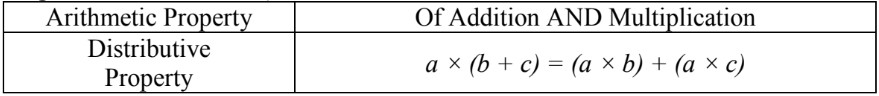
Arithmetic properties: Distributive property
Topic Notes
Notes:
- The distributive property is what happens when you multiply a number (called a multiplier or factor) with a sum of two or more numbers (addends inside of brackets).
- Ex. 2 × (9 + 5) =
- To distribute means to spread out or to hand around
- So, the distributive property makes you distribute the multiplier
- The multiplier/factor is distributed (given to) all the addends in brackets
- Ex. 2 × (9 + 5) = 2×9 + 2×5
- = 18 + 10 = 28
- In other words, multiplying a sum of two numbers is equal to the sum of each addend multiplied by the factor
- A common mistake that many students make with the distributive property is that they do not FULLY distribute the multiplier/factor:
- Ex. 2 × (9 + 5) the 2 should be multiplied with both addends = 2 × 9 + 2 × 5
- The common mistake is to only multiply the with the first addend:
- 2 × (9 + 5) ? 2 × 9 + 5
- 2 × 9 + 5 = 18 + 5 = 23
- The correct answer should have been 28; not distributing will give the incorrect answer of 23
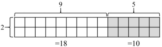
- The distributive property can be demonstrated using area block models:
- Area is given by two dimensions (i.e. length × width or height × length)
- Ex. 2 × (9 + 5) means an area block with a height of 2, and a combined length of 9 and 5. The total number of area blocks is 28.
- The general formula for the distributive property (where , and are variables that represent real numbers) is:
- The distributive property works for any type of real number as the multiplier and/or addends (such as integers, fractions, and/or decimals):
- Ex. -3 x
- Ex. 5 × (0.2+ 0.05) = (5×0.2) + (5×0.05) = 1.0 + 0.25 = 1.25
Introduction to the Distributive Property
The distributive property is a fundamental concept in arithmetic that plays a crucial role in simplifying mathematical expressions. As introduced in our video, this property demonstrates how multiplication can be distributed over addition. It states that multiplying a number by a sum is equivalent to multiplying the number by each addend separately and then adding the results. For example, a(b + c) = ab + ac. This property is not only essential in basic arithmetic but also forms the foundation for more advanced algebraic operations. Understanding the distributive property helps students solve complex problems more efficiently and provides a logical framework for manipulating equations. It's important to note that this property involves both addition and multiplication operations, making it a versatile tool in mathematical problem-solving. Mastering the distributive property is key to developing strong mathematical skills and reasoning abilities.
Understanding the Distributive Property
The distributive property in algebra is a fundamental concept in mathematics that allows us to simplify and solve complex equations. At its core, this property describes how multiplication interacts with addition or subtraction. To understand it better, let's use a simple analogy of distributing items to friends.
Imagine you have 3 bags, each containing 5 apples and 2 oranges. To find the total number of fruits, you could count all the apples and oranges in each bag separately. This would be like using the formula: 3 × (5 + 2). Alternatively, you could count all the apples from all bags, then all the oranges from all bags, and add these totals together. This represents the distributive property in algebra in action: 3 × 5 + 3 × 2.
The general formula for the distributive property is A(B + C) = AB + AC. Here's what each component means:
- A is the multiplier (in our example, the number of bags)
- B and C are the addends (in our example, the number of apples and oranges in each bag)
- (B + C) represents the sum inside the parentheses
- AB and AC represent the multiplier distributed to each addend
To apply the distributive property, follow these steps:
- Identify the multiplier (the number outside the parentheses)
- Identify the addends (the numbers inside the parentheses)
- Multiply the multiplier by the first addend
- Multiply the multiplier by the second addend
- Add the results of steps 3 and 4
Let's practice with another example: 4(6 + 3). Following our steps:
- The multiplier is 4
- The addends are 6 and 3
- 4 × 6 = 24
- 4 × 3 = 12
- 24 + 12 = 36
Therefore, 4(6 + 3) = 4 × 6 + 4 × 3 = 24 + 12 = 36.
The solving equations with distributive property is not just useful for simplifying expressions; it's also a powerful tool in mental math. For instance, when multiplying 7 × 98, you can rewrite it as 7(100 - 2). Using the distributive property, this becomes 700 - 14, which is easier to calculate mentally.
It's important to note that the solving equations with distributive property works with subtraction as well. The formula A(B - C) = AB - AC follows the same principle. For example, 5(8 - 3) can be rewritten as 5 × 8 - 5 × 3 = 40 - 15 = 25.
In algebra, the distributive property becomes even more crucial. It allows us to simplify expressions with variables, such as 2(x + 5) = 2x + 10. This property is essential in solving equations, factoring polynomials, and many other algebraic operations.
As you progress in mathematics, you'll find that the distributive property is a fundamental tool that appears in various contexts. From basic arithmetic to advanced calculus, this property remains a cornerstone of mathematical reasoning and problem-solving. By mastering the distributive property, you're building a strong foundation for more complex mathematical concepts and techniques.
Applying the Distributive Property with Area Models
Area models provide a powerful visual tool for understanding and applying the distributive property formula in mathematics. These models offer a concrete representation of abstract concepts, making it easier for learners to grasp the relationship between multiplication and addition. By using area models, we can effectively demonstrate how the distributive property works and why it's a fundamental principle in algebra.
In an area model for the distributive property, we create a rectangle where the multiplier represents the height, and the addends represent the length. This visual approach helps students see how multiplication can be broken down into smaller parts, which is the essence of the distributive property.
Let's consider a detailed example using whole numbers to illustrate this concept. Suppose we want to calculate 7 × (5 + 3). In this expression, 7 is our multiplier, and (5 + 3) represents the addends. To create an area model, we'll draw a rectangle with a height of 7 units and a length divided into two parts: 5 units and 3 units.
The resulting rectangle is split into two sections:
- The left section has an area of 7 × 5 = 35 square units
- The right section has an area of 7 × 3 = 21 square units
The total area of the rectangle is the sum of these two sections: 35 + 21 = 56 square units. This visual representation clearly shows that 7 × (5 + 3) is equal to (7 × 5) + (7 × 3), which is the essence of the distributive property.
This example directly relates to the distributive property formula: a(b + c) = ab + ac. In our case:
- a = 7 (the multiplier or height)
- b = 5 (the first addend or part of the length)
- c = 3 (the second addend or part of the length)
The area model visually proves that 7(5 + 3) = (7 × 5) + (7 × 3) = 35 + 21 = 56.
This visualization technique is particularly useful for understanding more complex expressions and can be extended to algebraic expressions with variables. For instance, we can use area models to represent expressions like 4(x + 2), where the height is 4, and the length is divided into x and 2 units.
By consistently using area models, students can develop a strong intuition for the distributive property and its applications in various mathematical contexts. This approach not only aids in solving multiplication problems but also lays a solid foundation for more advanced algebraic concepts.
The Distributive Property with Different Number Types
The distributive property is a fundamental concept in mathematics that applies to all real numbers, including integers, fractions, and decimals. This property states that multiplying a number by a sum is the same as multiplying the number by each addend and then adding the products. Let's explore how this property works with different types of real numbers.
For integers, the distributive property is straightforward. Consider the expression 3(4 + 5). Using the distributive property, we can rewrite this as (3 × 4) + (3 × 5). Let's solve it step-by-step:
- 3(4 + 5)
- (3 × 4) + (3 × 5)
- 12 + 15
- 27
This demonstrates that the distributive property holds true for integers. Now, let's look at how it applies to fractions. Consider the expression 1/2(3/4 + 2/3). We can apply the distributive property as follows:
- 1/2(3/4 + 2/3)
- (1/2 × 3/4) + (1/2 × 2/3)
- 3/8 + 1/3
- (9/24) + (8/24)
- 17/24
As we can see, the distributive property works equally well with fractions. The key is to perform the multiplication first, then add the resulting fractions using a common denominator.
For decimals, the distributive property follows the same principle. Let's examine the expression 0.5(1.2 + 0.8):
- 0.5(1.2 + 0.8)
- (0.5 × 1.2) + (0.5 × 0.8)
- 0.6 + 0.4
- 1.0
This example illustrates that the distributive property is equally applicable to decimal numbers. When working with decimals, it's important to align the decimal points correctly during addition.
The distributive property is not limited to these types of numbers; it works for all real numbers. This includes irrational numbers like π or 2. For instance, π(2 + 3) can be rewritten as (π × 2) + (π × 3).
Understanding the distributive property in algebra is crucial in algebra and higher mathematics. It allows us to simplify complex expressions, solve equations more efficiently, and manipulate algebraic expressions. For example, when factoring polynomials, we often use the distributive property in reverse, identifying common factors to simplify expressions.
In real-world applications, the distributive property is used in various fields. In economics, it's applied when calculating compound interest or determining price adjustments. In physics, it's used in vector calculations and force analysis. Even in everyday situations like shopping, we unconsciously use the distributive property when calculating discounts or comparing prices.
To further illustrate the universality of this property, consider a mixed number types distributive property example: 2(3.5 + 1/4). We can solve this using the distributive property:
- 2(3.5 + 1/4)
- (2 × 3.5) + (2 × 1/4)
- 7 + 1/2
- 7.5
This example combines integers, decimals, and fractions, demonstrating that the distributive property works seamlessly across different number types.
In conclusion, the distributive property in algebra is a powerful tool in mathematics that applies universally to all real numbers. Whether working with integers, fractions, or distributive property with irrational numbers, understanding this property is essential for solving equations and simplifying expressions.
Common Mistakes and How to Avoid Them
When applying the distributive property in mathematics, students often encounter several common mistakes that can lead to incorrect solutions. One of the most prevalent errors is distributing only to the first term, neglecting the subsequent terms in the expression. This oversight can significantly impact the accuracy of calculations and problem-solving.
For example, consider the expression 3(x + 2y - 4). A common mistake would be to distribute the 3 only to the first term, resulting in the incorrect solution 3x + 2y - 4. The correct application of the distributive property would yield 3x + 6y - 12. This error stems from a misunderstanding of the property's fundamental principle, which requires distribution to all terms within the parentheses.
Another frequent mistake is forgetting to distribute negative signs when dealing with subtraction. For instance, in the expression -(a + b), students might incorrectly write -a + b instead of the correct form -a - b. This error often occurs due to a lack of attention to the negative sign's impact on all terms within the parentheses.
To avoid these common mistakes, students can employ several strategies. First, it's crucial to visualize the distributive property as "multiplying each term inside the parentheses by the factor outside." This mental image can help reinforce the need to distribute to all terms. Additionally, using a systematic approach, such as drawing arrows from the outside factor to each term inside the parentheses, can serve as a visual reminder to distribute completely.
Another helpful tip is to always check your work by expanding the original expression and comparing it to your simplified version. This verification process can catch errors and reinforce correct application of the property. Moreover, practicing with a variety of expressions, including those with negative signs and multiple terms, can build confidence and proficiency in applying the distributive property accurately.
It's also beneficial to understand the underlying concept of the distributive property rather than merely memorizing rules. Recognizing that distribution is based on the idea of breaking down a complex multiplication into simpler, more manageable parts can provide a deeper understanding and reduce errors. By focusing on these strategies and being mindful of common pitfalls, students can significantly improve their ability to apply the distributive property correctly and avoid typical mistakes in their mathematical problem-solving.
Practical Applications of the Distributive Property
The distributive property, a fundamental concept in mathematics, has numerous real-world applications that extend far beyond the classroom. This property, which states that a(b + c) = ab + ac, proves invaluable in simplifying complex calculations and enhancing problem-solving efficiency in everyday situations. Let's explore how this mathematical principle applies to practical scenarios, particularly in cooking and finance.
In the culinary world, the distributive property often comes into play when scaling recipes. Imagine you're preparing a dish that serves four people, but you need to adjust it for a party of twelve. Instead of recalculating each ingredient separately, you can use the distributive property to simplify the process. For instance, if a recipe calls for 2 cups of flour, 1 cup of sugar, and 3 eggs, you can express the scaling as 3(2 cups flour + 1 cup sugar + 3 eggs) = 6 cups flour + 3 cups sugar + 9 eggs. This approach not only saves time but also reduces the likelihood of calculation errors.
Financial calculations provide another fertile ground for applying the distributive property. Consider a scenario where you're calculating the total cost of multiple items with a sales tax. If you're purchasing three items priced at $20, $30, and $50, with an 8% sales tax, you could calculate the tax on each item separately and then sum the results. However, using the distributive property, you can simplify this to 0.08($20 + $30 + $50) = 0.08($100) = $8. This method is not only quicker but also minimizes the chance of rounding errors that could occur when calculating tax on individual items.
The distributive property also proves useful in more complex financial scenarios, such as calculating compound interest or evaluating investment portfolios. When dealing with multiple investments or loans with varying interest rates, this property allows for more streamlined calculations and clearer comparisons between different financial products.
In the realm of problem-solving, understanding and applying the distributive property can lead to more efficient strategies. For example, mental math becomes significantly easier when you can break down complex calculations into simpler parts. If you need to multiply 25 by 18, you might use the distributive property to think of it as 25(20 - 2) = 25(20) - 25(2) = 500 - 50 = 450. This approach allows for quicker mental calculations by leveraging known facts (like 25 x 20 is easy to compute) and then adjusting the result.
The efficiency gained through the distributive property extends to various other fields as well. In computer programming, it's used to optimize code and improve algorithm performance. In physics and engineering, it simplifies complex equations, making them more manageable and easier to solve. Even in everyday tasks like budgeting or planning, the ability to distribute values across multiple categories can lead to more organized and accurate results.
By recognizing opportunities to apply the distributive property in real-world scenarios, individuals can enhance their problem-solving skills and tackle complex calculations with greater confidence and accuracy. Whether you're adjusting a recipe, managing finances, or solving intricate mathematical problems, this fundamental principle offers a powerful tool for simplification and efficiency. As we continue to encounter increasingly complex data and calculations in our daily lives, the ability to leverage mathematical properties like distribution becomes not just useful, but essential for navigating the modern world effectively.
Conclusion
In summary, the distributive property is a fundamental concept in mathematics, allowing us to simplify and solve complex equations. This property states that multiplying a number by a sum is equivalent to multiplying the number by each addend and then adding the products. Its importance in arithmetic and algebra cannot be overstated, as it forms the basis for many advanced mathematical operations. We encourage you to practice applying the distributive property in various contexts, from basic arithmetic to algebraic expressions, to solidify your understanding. Remember, the introduction video provides a strong foundation, but continued practice is key to mastery. For further learning, explore online resources, textbooks, and practice problems to enhance your skills. By mastering the distributive property, you'll unlock new problem-solving strategies and gain a deeper appreciation for mathematical relationships. Keep practicing, and you'll soon find yourself confidently applying this essential property across diverse mathematical scenarios.
Introduction to the Distributive Property
In this lesson, we will explore the distributive property, an essential arithmetic property that combines both multiplication and addition. The distributive property states that multiplying a number by a sum of two addends is equivalent to multiplying the number by each addend separately and then adding the results. This can be expressed as .
Step 1: Understanding the Distributive Property
The distributive property is unique because it involves two operations: multiplication and addition. Unlike other properties that focus on a single operation, the distributive property shows how multiplication can be distributed over addition. This means that when you have a number multiplying a sum, you can distribute the multiplication to each addend within the sum.
Step 2: Setting Up the Example
Let's consider an example to illustrate the distributive property. Suppose we have the expression . Here, 2 is the multiplier, and 9 and 5 are the addends grouped together within the parentheses. Our goal is to apply the distributive property to simplify this expression.
Step 3: Applying the Distributive Property
According to the distributive property, we need to distribute the multiplier (2) to each addend (9 and 5) separately. This means we will perform the following operations:
- Multiply 2 by 9
- Multiply 2 by 5
So, the expression can be rewritten as .
Step 4: Performing the Multiplications
Next, we perform the multiplications:
So, the expression simplifies to .
Step 5: Adding the Results
Finally, we add the results of the multiplications:
Therefore, when we apply the distributive property.
Step 6: Verifying the Result
To verify our result, we can solve the original expression using the order of operations (also known as BEDMAS or PEMDAS). First, we perform the addition inside the parentheses:
Then, we multiply the result by 2:
As expected, we get the same result, confirming that our application of the distributive property was correct.
Step 7: Generalizing the Distributive Property
The distributive property can be generalized for any numbers , , and . It shows that multiplying a sum of two numbers by a factor is equal to the sum of each addend multiplied by the same factor. Mathematically, this is expressed as:
This property is fundamental in arithmetic and algebra, making it easier to simplify and solve complex expressions.
FAQs
-
What is the distributive property?
The distributive property is a fundamental mathematical concept that states multiplying a number by a sum is equivalent to multiplying the number by each addend and then adding the products. In algebraic form, it's expressed as a(b + c) = ab + ac.
-
How does the distributive property work with negative numbers?
The distributive property works the same way with negative numbers. For example, -2(3 + 4) = (-2 × 3) + (-2 × 4) = -6 + (-8) = -14. It's important to remember that the negative sign distributes to all terms inside the parentheses.
-
Can the distributive property be used with variables?
Yes, the distributive property applies to variables as well as numbers. For instance, x(y + z) = xy + xz. This makes it a powerful tool in algebra for simplifying expressions and solving equations.
-
How is the distributive property used in real-life situations?
The distributive property is often used in everyday calculations, such as determining sales tax on multiple items, adjusting recipes for different serving sizes, or calculating discounts on purchases. It simplifies complex calculations by breaking them down into manageable parts.
-
What's the difference between the distributive property and the associative property?
While both are important mathematical properties, they serve different purposes. The distributive property involves distributing multiplication over addition or subtraction (a(b + c) = ab + ac), whereas the associative property states that the grouping of factors in multiplication doesn't affect the product ((a × b) × c = a × (b × c)).
Prerequisite Topics
Understanding the distributive property in arithmetic is crucial for advancing in mathematics, but it's equally important to recognize how this concept builds upon and relates to other fundamental topics. To fully grasp the distributive property, students should have a solid foundation in several key areas.
One essential prerequisite is simplifying mathematical expressions. This skill is vital because the distributive property often involves simplifying expressions after distribution. Being able to manipulate and simplify rational expressions provides the necessary groundwork for applying the distributive property effectively.
Another important prerequisite is solving linear equations. The distributive property is frequently used in solving linear equations, especially those involving distance and time. Understanding how to apply this property can significantly simplify complex problems and make them more manageable.
Factoring polynomials is also closely related to the distributive property. In fact, the distributive property is the reverse process of factoring. When students understand how to factor polynomials, they can more easily grasp how the distributive property works in expanding expressions.
Interestingly, even topics that might seem unrelated at first glance can be relevant. For instance, calculating compound interest in finance often involves applying the distributive property to simplify complex formulas. This demonstrates how the distributive property extends beyond basic arithmetic and algebra into real-world applications.
By mastering these prerequisite topics, students build a strong foundation for understanding the distributive property. This property is not an isolated concept but rather a crucial link in the chain of mathematical reasoning. It connects basic arithmetic operations to more advanced algebraic concepts and has wide-ranging applications in various fields of mathematics and beyond.
The distributive property serves as a bridge between simpler mathematical operations and more complex problem-solving techniques. It allows for the simplification of expressions, solving of equations, and manipulation of algebraic structures. By recognizing its relationship to other mathematical concepts, students can develop a more comprehensive and interconnected understanding of mathematics as a whole.
In conclusion, while focusing on the distributive property itself is important, it's equally crucial to understand and appreciate its connections to other mathematical concepts. This holistic approach not only enhances understanding of the distributive property but also reinforces the interconnected nature of mathematics, preparing students for more advanced topics and real-world applications.