0/4
?
Intros
Lessons
  1. Riemann Sum overview:
  2. area under the curve
  3. summation formula
  4. what is "Riemann Sum"?
  5. integrals expressed as Riemann Sum
0/7
?
Examples
Lessons
  1. Finding the area under the graph of a function using a graphing calculator.
    Consider the function f(x)=x2f\left( x \right) = {x^2}, 1x31 \le x \le 3.
    Find the area under the graph of ff using a graphing calculator.
    1. Finding the area under the graph of a function using the Riemann Sum.
      Consider the function f(x)=x2f\left( x \right) = {x^2}, 1x31 \le x \le 3.
      Estimate the area under the graph of ff using four approximating rectangles and taking the sample points to be:
      1. right endpoints
      2. left endpoints
      3. midpoints
    2. Evaluating integrals with a Riemann Sum
      Consider the function f(x)=x25x+3f\left( x \right) = {x^2} - 5x + 3, 2x52 \le x \le 5.
      1. Evaluate the Right Riemann sum for ff with 6 sub-intervals.
      2. Evaluate 25(x25x+3)dx\int_2^5 \left( {{x^2} - 5x + 3} \right)dx, by finding the Riemann sum for ff with \infty intervals.
    3. Evaluating Riemann Sum with trapezoids
      Consider the function f(x)=x2f\left( x \right) = {x^2}, 1x31 \le x \le 3. Estimate the area under the graph of ff using four approximating trapezoids.
      Topic Notes
      ?
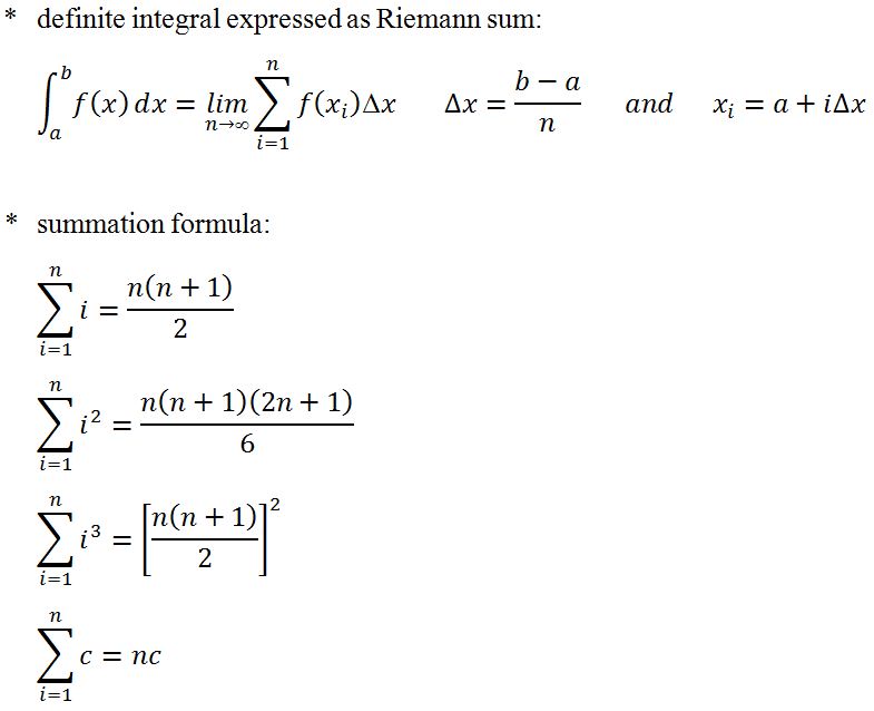
      In this lesson, we will learn how to approximate the area under the curve using rectangles. First we notice that finding the area under the curve is easy if the function is a straight line. However, what if it is a curve? We will actually have to approximate curves using a method called "Riemann Sum". This method involves finding the length of each sub-interval (delta x), and finding the points of interest, finding the y values of each point of interest, and then use the find the area of each rectangle to sum them up. There are 3 methods in using the Riemann Sum. First is the "Right Riemann Sum", second is the "Left Riemann Sum", and third is the "Middle Riemann Sum". Lastly, we will look at the idea of infinite sub-intervals (which leads to integrals) to exactly calculate the area under the curve.

      Introduction to Riemann Sum

      Welcome to our exploration of Riemann sum, a fundamental concept in calculus that's essential for understanding area under the curve and integral calculus. Named after the brilliant mathematician Bernhard Riemann, this method provides a powerful way to approximate the area of complex shapes by breaking them down into simpler geometric forms. As we dive into this topic, you'll discover how Riemann sum serves as a bridge between basic geometry and advanced calculus, offering a practical approach to solving real-world problems. Our introduction video will guide you through the basics, demonstrating how to construct Riemann sums and interpret their results. You'll see firsthand how this approximation technique evolves into the more precise methods of integration. Whether you're new to calculus or looking to reinforce your understanding, mastering Riemann sum will equip you with a valuable tool for analyzing curves and functions. Let's embark on this mathematical journey together and unlock the power of Riemann sum in calculus!

      Understanding Area Under the Curve

      The concept of "area under the curve" is a fundamental principle in calculus that plays a crucial role in various mathematical and real-world applications. It's a method used to calculate the area between a function's graph and the x-axis within a specific interval. This concept is essential because it helps us understand and quantify accumulated change over time or space, which is vital in fields like physics, economics, and engineering.

      Let's start with a simple example to illustrate this concept. Consider the linear function y = x. Imagine we want to find the area under this line from x = 0 to x = 2. In this case, we're dealing with a straight line, so the area forms a triangle. We can easily calculate this area using the formula for a triangle's area: (base * height) / 2. Here, the base is 2, and the height is also 2, so the area is (2 * 2) / 2 = 2 square units.

      This straightforward calculation works well for linear functions, but what happens when we encounter a curve? That's where the real challenge begins, and it's why the concept of area under the curve is so important in calculus. Let's consider the nonlinear function y = x^2. The area under this curve can't be calculated using simple geometric formulas because the curve's height is constantly changing.

      To tackle this problem, mathematicians developed a clever approach. They divide the area under the curve into many thin rectangles. The more rectangles we use, the more accurate our approximation becomes. Here's how it works step-by-step:

      1. Divide the interval on the x-axis into many small segments.
      2. For each segment, create a rectangle that reaches up to the curve.
      3. Calculate the area of each rectangle (width * height).
      4. Sum up all these rectangular areas.

      As we increase the number of rectangles, making them thinner and thinner, our sum gets closer and closer to the true area under the curve. In calculus, we take this process to its logical extreme, using infinitely many infinitely thin rectangles. This is where the concept of integration comes in, allowing us to calculate the exact area under curves like y = x^2.

      The beauty of this method is that it works for any function, not just simple ones like y = x or y = x^2. It allows us to calculate areas under complex curves that would be impossible to determine using elementary geometry. This technique is invaluable in many practical applications, such as:

      • Calculating the total distance traveled by an object given its velocity over time.
      • Determining the work done by a variable force.
      • Computing probabilities in statistics.
      • Analyzing consumer surplus in economics.

      Understanding the area under the curve is like having a superpower in mathematics. It allows us to solve problems that would otherwise be intractable. While the concept might seem abstract at first, with practice and real-world examples, you'll start to see its applications everywhere.

      Remember, whether you're dealing with a simple linear function like y = x or a more complex curve like y = x^2, the principle remains the same. We're always trying to quantify the accumulated change represented by the area between the function and the x-axis. As you continue your journey in calculus, you'll discover even more powerful tools and techniques built upon this fundamental concept.

      Introduction to Riemann Sum Approximation

      Welcome to the fascinating world of Riemann sums! If you've ever wondered how mathematicians approximate the area under a curve, you're in for a treat. The Riemann sum is a powerful method that uses rectangles to estimate the area beneath a function's graph. Let's dive in and explore this concept together!

      Imagine you're trying to measure the area of an oddly shaped field. One way to do this would be to divide the field into smaller, more manageable rectangles and add up their areas. This is essentially what a Riemann sum does, but with mathematical functions instead of fields.

      Let's use a concrete example to illustrate this concept. Consider the function y = x^2 from x = 0 to x = 2. We want to approximate the area under this curve using rectangles. Here's where the magic of Riemann sums comes into play!

      To start, we divide the interval [0, 2] into smaller subintervals. The width of each subinterval is called delta x (Δx). For instance, if we use four rectangles, Δx would be (2 - 0) / 4 = 0.5.

      Next, we need to determine the height of each rectangle. This is where xi and f(xi) come in. xi represents a point within each subinterval, and f(xi) is the function value at that point. Depending on where we choose xi, we can get different approximations:

      1. Left endpoint: xi is at the left of each subinterval
      2. Right endpoint: xi is at the right of each subinterval
      3. Midpoint: xi is at the center of each subinterval

      Now, let's talk about overestimation and underestimation. When we use left endpoints for a function that's increasing and concave up (like our x^2 example), we tend to underestimate the true area. Conversely, using right endpoints in this case would lead to an overestimation. The midpoint method often provides a more balanced approximation.

      Ready to calculate? Here's a step-by-step guide to finding the Riemann sum:

      1. Calculate Δx: Divide the interval length by the number of rectangles
      2. Determine xi for each subinterval based on your chosen method (left, right, or midpoint)
      3. Calculate f(xi) for each xi
      4. Multiply each f(xi) by Δx to get the area of each rectangle
      5. Sum up all these areas to get your Riemann sum approximation

      For our y = x^2 example from 0 to 2 using four rectangles and left endpoints:

      • Δx = (2 - 0) / 4 = 0.5
      • xi values: 0, 0.5, 1, 1.5
      • f(xi) values: 0, 0.25, 1, 2.25
      • Riemann sum = 0.5 * (0 + 0.25 + 1 + 2.25) = 1.75

      This underestimates the true area, which is actually 8/3 2.67. As you increase the number of rectangles, your approximation gets closer to the true value!

      Riemann sums are not just a mathematical curiosity; they form the foundation for integral calculus and have practical applications in physics, engineering, and economics. By mastering this concept, you're opening doors to understanding more advanced mathematical ideas.

      Remember, practice makes perfect! Try calculating Riemann sums with different functions, intervals, and numbers of rectangles. As you become more comfortable with the process, you'll gain a deeper appreciation for this powerful approximation method. Happy

      Types of Riemann Sum

      When it comes to approximating the area under a curve, Riemann sums are incredibly useful tools. There are three main types of Riemann sums: Left Riemann Sum, Right Riemann Sum, and Middle Riemann Sum. Let's explore each of these methods and see how they affect the accuracy of our approximations.

      First, let's talk about the Left Riemann Sum. In this method, we use the leftmost point of each subinterval to calculate the height of our rectangles. Imagine we're trying to approximate the area under a curve representing the speed of a car over time. If we use the Left Riemann Sum, we're essentially assuming the car maintains its initial speed for each time interval. This can lead to an underestimation of the total distance traveled if the speed is generally increasing, or an overestimation if it's decreasing.

      Next, we have the Right Riemann Sum. As you might guess, this method uses the rightmost point of each subinterval. In our car example, this would be like assuming the car maintains its final speed for each time interval. The Right Riemann Sum tends to overestimate the area when the function is increasing and underestimate when it's decreasing the opposite of the Left Riemann Sum.

      Finally, we have the Middle Riemann Sum. This method takes a middle ground approach by using the midpoint of each subinterval to determine the rectangle heights. In our car analogy, this would be like assuming the car maintains its average speed for each time interval. The Middle Riemann Sum often provides a more accurate approximation than either the Left or Right Riemann Sum, especially when the function is relatively smooth.

      So, how do these methods affect the accuracy of our approximations? Well, it largely depends on the shape of the function we're working with. For a strictly increasing function, the Left Riemann Sum will always underestimate the true area, while the Right Riemann Sum will overestimate it. The opposite is true for a strictly decreasing function. The Middle Riemann Sum tends to balance out these over- and underestimations, often resulting in a more accurate approximation.

      However, it's important to note that regardless of which method we use, the accuracy of our approximation improves as we increase the number of subintervals. This is because smaller subintervals mean our rectangles more closely match the shape of the curve. In fact, as the number of subintervals approaches infinity, all three methods converge to the true value of the definite integral.

      To illustrate this, let's consider a simple example. Imagine we're approximating the area under the curve y = x² from 0 to 2. If we use just four subintervals, we might get quite different results with each method. The Left Riemann Sum might give us 2.75, the Right Riemann Sum 4.75, and the Middle Riemann Sum 3.5. The true value is actually 8/3 (approximately 2.67). As we increase the number of subintervals, all these approximations will get closer to the true value of the definite integral.

      In practice, the choice between these methods often depends on the specific problem and the level of accuracy required. Sometimes, we might even use a combination of methods to get upper and lower bounds for our approximation. Remember, the key to mastering Riemann sums is practice and understanding how the shape of the function affects our approximations. Keep experimenting with different functions and methods, and you'll soon develop a strong intuition for this powerful mathematical tool!

      Summation Notation and Formulas

      Let's dive into the world of summation notation and its crucial role in Riemann sum calculations! Summation notation, often represented by the Greek letter Sigma (Σ), is a powerful mathematical shorthand that allows us to express the sum of a sequence of numbers concisely. This notation is particularly useful when dealing with Riemann sums, which are fundamental in calculus for approximating the area under a curve.

      In the context of Riemann sums, summation notation helps us represent the sum of many rectangular areas efficiently. Instead of writing out each term individually, we can use a single expression to represent the entire sum. For example, the formula Σ(f(xi)Δx) from i=1 to n succinctly represents the Riemann sum of a function f(x) over n subintervals.

      Now, let's review some key summation formulas that can significantly simplify our Riemann sum calculations. Two particularly useful formulas are the sum of i and the sum of i2 from 1 to n:

      1. Sum of i: Σi = n(n+1)/2
      2. Sum of i2: Σi2 = n(n+1)(2n+1)/6

      These formulas are incredibly handy because they allow us to quickly compute sums that would otherwise require tedious calculations, especially when dealing with large values of n. By memorizing and understanding these formulas, you can save valuable time and reduce the likelihood of errors in your calculations.

      Let's see how these formulas can be applied in practice. Imagine we're calculating a Riemann sum where the height of each rectangle is given by f(xi) = 2i + 1, and we're using n = 100 subintervals over the interval [0, 1]. The width of each subinterval, Δx, would be 1/100.

      Without using our summation formulas, we'd need to calculate:

      Σ(2i + 1)(1/100) for i from 1 to 100

      This would involve adding up 100 terms! However, using our summation formulas, we can simplify this:

      Σ(2i + 1)(1/100) = (1/100)[2Σi + Σ1]
      = (1/100)[2(100(101)/2) + 100]
      = (1/100)[10100 + 100]
      = 102

      As you can see, using the summation formula for Σi allowed us to quickly solve what would have been a time-consuming calculation. This example demonstrates how these formulas can dramatically simplify Riemann sum calculations, especially when dealing with large numbers of subintervals.

      Remember, practice makes perfect! The more you work with these formulas and apply them to various problems, the more comfortable and proficient you'll become. Don't be discouraged if it takes some time to get used to them everyone learns at their own pace.

      In conclusion, mastering summation notation and these key formulas will greatly enhance your ability to work with Riemann sums and other related concepts in calculus. They're valuable tools in your mathematical toolkit, helping you tackle complex problems with greater ease and efficiency. Keep practicing, and soon you'll find yourself breezing through calculations that once seemed daunting!

      From Riemann Sum to Integrals

      Let's embark on an exciting journey through the world of calculus, exploring the fascinating concept of infinite subintervals and how it leads us to the powerful idea of integrals. Imagine we're trying to calculate the area under a curve, specifically y = x² from x = 1 to x = 2. This seemingly simple task opens up a world of mathematical wonder!

      To begin, let's think about how we might approximate this area. We could start by dividing the interval [1, 2] into smaller subintervals and creating rectangles that roughly fit under the curve. The more rectangles we use, the closer our approximation gets to the true area. But what if we could use an infinite number of rectangles? This is where the magic of calculus comes into play!

      As we increase the number of subintervals, something remarkable happens. Our approximation becomes more and more accurate, and we can express this mathematically using a Riemann sum. The Riemann sum is the sum of the areas of all these rectangles. For our y = x² example, if we divide the interval into n equal subintervals, each with a width of Δx = (2 - 1) / n = 1 / n, we can write the Riemann sum as:

      Σ from i = 1 to n of f(x_i) * Δx

      Here, f(x_i) represents the height of each rectangle, which is the value of x² at a chosen point in each subinterval. As n approaches infinity, this sum gets closer and closer to the true area under the curve.

      Now, here's where it gets really interesting! As we let n approach infinity, our Riemann sum transforms into a limit. We express this as:

      lim as n of Σ from i = 1 to n of f(x_i) * Δx

      This limit is precisely what we call an integral! In our case, it would be written as:

      from 1 to 2 of x² dx

      This integral represents the exact area under the curve y = x² from x = 1 to x = 2. It's not just an approximation anymore; it's the true value we've been seeking!

      The transition from Riemann sum to integral is a pivotal moment in calculus. It allows us to move from discrete approximations to continuous, exact calculations. This concept opens up a whole new world of possibilities in mathematics and its applications.

      With integrals, we can now calculate areas under curves, volumes of complex shapes, work done by varying forces, and so much more. The beauty of this transition lies in its ability to bridge the gap between the finite and the infinite, giving us a tool to understand and quantify continuous change.

      In our everyday lives, we often encounter situations where things change continuously like the speed of a car, the growth of a population, or the flow of a river. Integrals provide us with a powerful way to analyze and make sense of these continuous changes.

      As we've seen with our y = x² example, the process of moving from a Riemann sum to an integral involves taking a limit as the number of subintervals approaches infinity. This limit allows us to capture the cumulative effect of infinitesimal changes, which is at the heart of calculus.

      The significance of this transition extends far beyond just calculating areas. It forms the foundation for solving differential equations, understanding physics principles, and modeling complex systems in fields ranging from engineering to economics.

      So, the next time you see an integral symbol, remember the journey we've taken from approximating with finite rectangles to capturing the true area with an infinite number of infinitesimally thin rectangles. It's a beautiful example of how mathematics allows us to grasp and work with concepts that stretch beyond our immediate physical intuition.

      As we continue to explore calculus, keep this fundamental idea in mind. The transition from Riemann sums to integrals is not just a mathematical trick; it's a powerful conceptual leap that allows us to understand and quantify the differential equations.

      Conclusion

      In this article, we've explored the fundamental concept of Riemann sum and its crucial role in understanding integrals. We've seen how this mathematical tool allows us to approximate the area under a curve by dividing it into smaller, more manageable sections. The introduction video provided visual and practical examples, making the concept more accessible and relatable. Remember, Riemann sum is not just a theoretical concept but a practical tool used in various fields, from physics to economics. As you continue your mathematical journey, practice solving Riemann sum problems to reinforce your understanding. Don't hesitate to explore additional resources to deepen your knowledge. Math can be challenging, but with persistence and the right approach, you'll master these concepts. Keep up the great work, and remember that each step forward in understanding brings you closer to mathematical proficiency. Stay curious and keep exploring the fascinating world of calculus!

      Riemann Sum Overview: Area Under the Curve

      In this guide, we will explore the concept of Riemann Sum and how it helps in approximating the area under a curve. We will break down the process step by step to ensure a clear understanding of the topic.

      Step 1: Understanding the Area Under the Curve

      Before diving into Riemann Sum, it's essential to understand the concept of the area under the curve. The area under the curve represents the integral of a function over a specified interval. For instance, if we want to find the area under the curve from -1 to 4, we need to consider the region between these points on the x-axis.

      To visualize this, imagine a curve on a graph. The area under this curve from -1 to 4 is the region bounded by the curve, the x-axis, and the vertical lines at x = -1 and x = 4. This area can be divided into simpler geometric shapes, such as triangles, to facilitate calculation.

      Step 2: Calculating the Area Using Triangles

      Let's start by calculating the area under the curve y = x from 0 to 4. This region forms a right triangle with the x-axis. The base of the triangle is 4 units (from 0 to 4), and the height is also 4 units (since y = x at x = 4).

      The area of a triangle is given by the formula:

      Area = (Base × Height) / 2

      Substituting the values, we get:

      Area = (4 × 4) / 2 = 16 / 2 = 8

      So, the area of the triangle from 0 to 4 is 8 square units.

      Step 3: Considering the Negative Side of the Graph

      Next, we need to calculate the area from -1 to 0. This region also forms a right triangle, but it lies below the x-axis. The base and height of this triangle are both 1 unit.

      Using the same formula for the area of a triangle:

      Area = (1 × 1) / 2 = 1 / 2 = 0.5

      Since this area is below the x-axis, it is considered negative. Therefore, the area from -1 to 0 is -0.5 square units.

      Step 4: Summing the Areas

      To find the total area under the curve from -1 to 4, we sum the areas of the two triangles:

      Total Area = Area from 0 to 4 + Area from -1 to 0

      Total Area = 8 + (-0.5) = 8 - 0.5 = 7.5

      Thus, the total area under the curve y = x from -1 to 4 is 7.5 square units.

      Step 5: Introducing Riemann Sum for Nonlinear Functions

      While the above method works well for linear functions, it becomes challenging for nonlinear functions like y = x². In such cases, we use Riemann Sum to approximate the area under the curve.

      Riemann Sum involves dividing the area under the curve into small rectangles and summing their areas. The more rectangles we use, the more accurate our approximation becomes.

      Step 6: Approximating Area Using Rectangles

      Consider the function y = x² and the interval from 0 to 2. To approximate the area under the curve, we divide this interval into smaller subintervals and draw rectangles within each subinterval.

      For example, we can divide the interval [0, 2] into four subintervals: [0, 0.5], [0.5, 1], [1, 1.5], and [1.5, 2]. For each subinterval, we draw a rectangle whose height is determined by the function value at the left endpoint of the subinterval.

      The area of each rectangle is given by:

      Area = Width × Height

      Summing the areas of all rectangles gives us an approximation of the total area under the curve.

      Step 7: Refining the Approximation

      To improve the accuracy of our approximation, we can increase the number of rectangles. As the number of rectangles approaches infinity, the Riemann Sum converges to the exact area under the curve, which is the definite integral of the function.

      In summary, Riemann Sum provides a method to approximate the area under a curve, especially for nonlinear functions. By dividing the interval into smaller subintervals and summing the areas of rectangles, we can estimate the total area with increasing accuracy.

      FAQs

      1. What is a Riemann sum?

        A Riemann sum is a method used to approximate the area under a curve by dividing it into smaller rectangles. It's named after the mathematician Bernhard Riemann and is a fundamental concept in calculus for understanding integrals.

      2. What are the different types of Riemann sums?

        There are three main types of Riemann sums: Left Riemann Sum (using the leftmost point of each subinterval), Right Riemann Sum (using the rightmost point), and Middle Riemann Sum (using the midpoint). Each type can lead to different approximations of the area under a curve.

      3. How does a Riemann sum relate to integrals?

        Riemann sums are the foundation for understanding integrals. As the number of rectangles in a Riemann sum approaches infinity, the sum approaches the exact value of the definite integral. This concept bridges the gap between discrete approximations and continuous calculations.

      4. What are some practical applications of Riemann sums?

        Riemann sums have various real-world applications, including calculating the distance traveled by an object given its velocity over time, determining work done by a variable force, computing probabilities in statistics, and analyzing consumer surplus in economics.

      5. How can I improve my understanding of Riemann sums?

        To improve your understanding of Riemann sums, practice calculating them with different functions, intervals, and numbers of rectangles. Visualize the process by drawing or using graphing software. Also, study the relationship between Riemann sums and integrals to grasp the bigger picture in calculus.

      Prerequisite Topics for Understanding Riemann Sum

      Before delving into the complex world of Riemann sums, it's crucial to have a solid foundation in several key mathematical concepts. Understanding these prerequisite topics will not only make learning about Riemann sums easier but also provide a deeper appreciation for its applications in calculus and beyond.

      One of the fundamental concepts you should be familiar with is applications of linear relations. Linear functions form the basis for many mathematical models and are essential in approximating curves, which is at the heart of Riemann sums. By understanding how linear relations can be applied to real-world situations, you'll be better equipped to grasp the concept of using rectangles to estimate the area under a curve.

      Another critical prerequisite is the definite integral. Riemann sums are intimately connected to definite integrals, as they provide a method for approximating the area under a curve. The definite integral can be thought of as the limit of Riemann sums as the number of rectangles approaches infinity. Having a strong grasp of definite integrals will help you understand the motivation behind Riemann sums and their significance in calculus.

      Lastly, familiarity with modeling with differential equations can provide valuable context for the applications of Riemann sums. While not directly used in the calculation of Riemann sums, understanding how differential equations model real-world phenomena can help you appreciate the power of integration techniques, including Riemann sums, in solving complex problems.

      By mastering these prerequisite topics, you'll be well-prepared to tackle the concept of Riemann sums. You'll understand how to break down complex curves into simpler linear approximations, appreciate the connection between sums and integrals, and see how these mathematical tools can be applied to solve real-world problems. Remember, mathematics is a cumulative subject, and each new concept builds upon previous knowledge. Taking the time to solidify your understanding of these prerequisites will pay dividends as you progress in your study of calculus and encounter more advanced integration techniques.

      As you embark on your journey to understand Riemann sums, keep in mind that these prerequisite topics are not just stepping stones but integral parts of a larger mathematical landscape. They provide the context and tools necessary to fully appreciate the elegance and power of Riemann sums in approximating areas and solving complex problems. By building a strong foundation in these areas, you'll be well-equipped to tackle not only Riemann sums but also more advanced topics in calculus and mathematical analysis.


      definite integral expressed as riemann sum, and summation formula
      Basic Concepts
      ?