TOPIC
MY PROGRESS
Pug Score
0%
Best Streak
0 in a row
Study Points
+0
Overview
Practice
Watch
Read
Quiz
Next Steps
Get Started
Get unlimited access to all videos, practice problems, and study tools.
Back to Menu
Topic Progress
Pug Score
0%
Videos Watched
0/0
Best Practice
No score
Read
Not viewed
Best Quiz
No attempts
Best Streak
0 in a row
Study Points
+0
Overview
Practice
Watch
Read
Quiz
Next Steps
Read
Taylor and maclaurin series
In this lesson, we will learn that most functions can be expressed as a Taylor Series. These are power series with a special form, and are centred at a point. If it is centred at 0, then it is called a Maclaurin Series. All of these series require the n'th derivative of the function at point a. We will first apply the Taylor Series formula to some functions. You may notice that trying to find a Taylor Series of a polynomial will just give us back the same polynomial, and not a power series. Then we will learn how to manipulate some of the formulas for some harder functions. Lastly, we will find the Taylor series for sine and cosine, which will requires us to recognize some patterns.
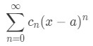
A power series is basically a series with the variable x in it. Formally speaking, the power series formula is:
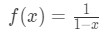
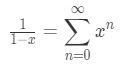
where \(c_{n}\) are the coefficients of each term in the series and \(a\) is a constant. Power series are important because we can use them to represent a function. For example, the power series representation of the function \(f(x) = \frac{1}{(1-x)} (for |x|\) < \(1)\) is:
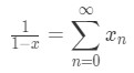
where \(a = 1\) and \(c_{n} = 1\).However, what if I want to find a power series representation for the integral of \(\frac{1}{(1-x)}\)? All you have to do is integrate the power series.
Question 1: Find a power series representation for the integral of the function
-
Equation 1: Power Series Representation integral pt.1 Recall that earlier we said that:
Equation 1: Power Series Representation integral pt.2 So if we integrate both sides, then we get:
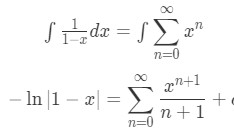
Equation 1: Power Series Representation integral pt.3 To find \(c\), we set \(x=0\). So we have:
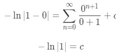
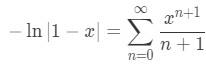
Equation 1: Power Series Representation integral pt.4 Notice that \(\ln (1)\) is equal to 0. So we get:

Equation 1: Power Series Representation integral pt.5 Hence we can conclude that:
Equation 1: Power Series Representation integral pt.6 If you want, you can make the series start at \(n=1\) instead, making the series become:
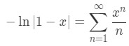
Equation 1: Power Series Representation integral pt.7
So what exactly are Taylor Series? If possible (not always), we can represent a function \(f(x)\) about \(x=a\) as a Power Series in the form:
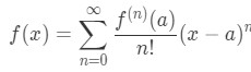
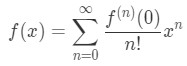
where \(f^{n} (a)\) is the \(n^{th}\) derivative about \(x = a\). This is the Taylor Series formula. If it is centred around \(x = 0\), then we call it the Maclaurin Series. Maclaurin Series are in the form:
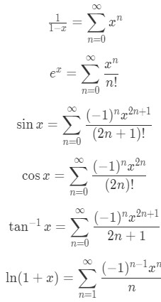
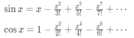
Here are some commonly used functions that can be represented as a Maclaurin Series:
We will learn how to use the Taylor Series formula later to get the common series, but first let's talk about Taylor Series Expansion.
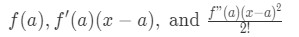
Of course if we expand the Taylor series out, we will get:

This is known as the Taylor Expansion Formula. We can use this to compute an infinite number of terms for the Taylor Series.
For example, let's say I want to compute the first three terms of the Taylor Series \(e^{x}\) about \(x = 1\).
Question 2: Find the first three terms of the Taylor Series for \(f(x) = e^{x}\).
- We will use the Taylor Series Expansion up to the third term. In other words, the first three terms are:
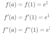
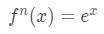
Equation 2: Taylor Expansion terms of e^x pt.1 Note that this is centred about \(x = 1\), hence we know

Equation 2: Taylor Expansion terms of e^x pt.2 We also know that taking derivatives gives us:
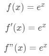
Equation 2: Taylor Expansion terms of e^x pt.3 Hence plugging \(a\) into each of these functions will give us:
Equation 2: Taylor Expansion terms of e^x pt.4 So we know that the first three terms are:
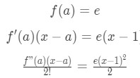
Equation 2: Taylor Expansion terms of e^x pt.5
Instead of finding the first three terms of the Taylor series, what if I want to find all the terms? In other words, can I find the Taylor Series which can give me all the terms? This is possible; however it can be difficult because you need to notice the pattern. Let's try it out!
Question 3: Find the Taylor Series of \(f(x) = e^{x}\) at \(x = 1\).
- Recall that the Taylor Expansion is:
Equation 3: Taylor Series of e^x pt.1 We know the first three terms, but we don't know any terms after. In fact, there are an infinite amount of terms after the third term. So how is it possible to figure what the term is when \(n \)→\( \infty\)? Well, we look for the pattern of the derivatives. If we are able to spot the patterns, then we will be able to figure out the \(n^{th}\) derivative is. Let's take a few derivatives first. Notice that:
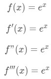
Equation 3: Taylor Series of e^x pt.2 The more derivatives you take, the most you realize that you will just get \(e^{x}\) back. Hence we can conclude that the \(n^{th}\) derivative is:
Equation 3: Taylor Series of e^x pt.3 Furthermore we know at \(a = 1\), hence
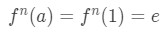
Equation 3: Taylor Series of e^x pt.4 Therefore plugging this in into the Taylor Series Formula gives:
Equation 3: Taylor Series of e^x pt.5 Notice that this Taylor Series for \(e^{x}\) is different from the Maclaurin Series for \(e^{x}\). This is because this one is centred at \(x=1\), while the other is centred around \(x=0\).You may have noticed that finding the \(n^{th}\) derivative was really easy here. What if the \(n^{th}\) derivative was not so easy to spot?
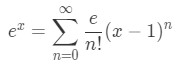
Question 4: Find the Taylor Series of \(f(x) = \sin x\) centred around \(a = 0\).
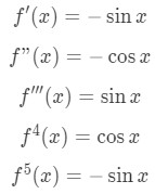
- Notice that if we take a few derivatives, we get:
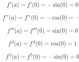
Equation 4: Taylor Series of sinx pt.1 Now the \(n^{th}\) derivative is not easy to spot here because the derivatives keep switching from cosine to sine. However, we do notice that the \(4^{th}\) derivative goes back \(\sin x\) again. This means that if we derive more after the \(4^{th}\) derivative, then we are going to get the same things again. We may see the pattern, but it doesn't tell us much about the \(n^{th}\) derivative. Why don't we plug \(a = 0\) into the derivatives?
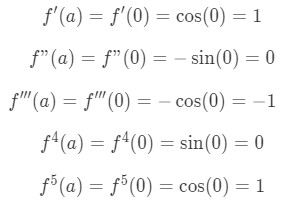
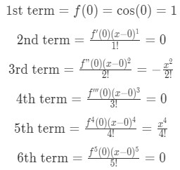
Equation 4: Taylor Series of sinx pt.2 Now we are getting something here. The values of the \(n^{th}\) derivative are always going to be 0, -1, or 1. Let's go ahead and find the first six terms of the Taylor Series using these derivative.
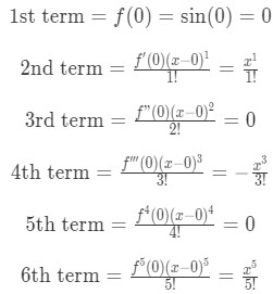
Equation 4: Taylor Series of sinx pt.3 If we are to add all the terms together (including term after the sixth term), we will get:
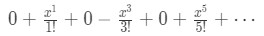
Equation 4: Taylor Series of sinx pt.4 This is the Taylor Expansion of \(\sin x\). Notice that every odd term is 0. In addition, every second term has interchanging signs. So we are going to rewrite this equation to:
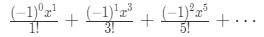
Equation 4: Taylor Series of sinx pt.5 Even though we have these three terms, we can pretty much see the patterns of where this series is going. The powers of \(x\) are always going to be odd. So we can generalize the powers to be \(2n+1\). The factorials are also always odd. So we can generalize the factorials to be \(2n+1\). The powers of -1 always go up by 1, so we can generalize that to be \(n\). Hence, we can write the Taylor Series \(\sin x\) as
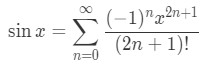
Equation 4: Taylor Series of sinx pt.6 which is a very common Taylor series. Note that you can use the same strategy when trying to find the Taylor Series for \(y = \cos x\).
Question 5: Find the Taylor Series of f(x) = cosx centred around.
- Notice that if we take a few derivatives, we get:
Equation 5: Taylor Series of cosx pt.1 Again, the \(n^{th}\) derivative is not easy to spot here because the derivatives keep switching from cosine to sine. However, we do notice that the \(4^{th}\) derivative goes back \(\cos x\) again. This means if we derive more after the \(4^{th}\) derivative, then we are going to get a loop. Now plugging in \(a=0\) we have
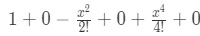
Equation 5: Taylor Series of cosx pt.2 Again, the values of the \(n^{th}\) derivative are always going to be 0, -1, or 1. Let's find the first six terms of the Taylor Series using the derivatives from above.
Equation 5: Taylor Series of cosx pt.3 If we are to add all the terms together (including term after the sixth term), we will get:
Equation 5: Taylor Series of cosx pt.4 Notice that this time all even terms are 0 and every odd term have interchanging signs. So we are going to rewrite this equation to:
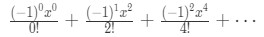
Equation 5: Taylor Series of cosx pt.5 We pretty much know the pattern here. The powers of x are always even. So we can generalize the powers to be \(2n\). The factorials are always even, so we can generalize them to be \(2n\). Lastly, the powers of -1 goes up by 1. So we can generalize that to be n. Hence, we can write the Taylor Series \(\cos x\) as:
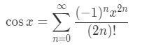
Equation 5: Taylor Series of cosx pt.6
- Notice that the Maclaurin Series of \(\cos x\) and \(\sin x\) are very similar. In fact, they only defer by the powers. If we were to expand the Taylor series of \(\cos x\) and \(\sin x\), we see that:
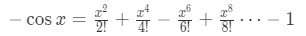
Equation 6: Taylor Expansion Relationship cosx and sinx pt.1 We can actually find a relationship between these two Taylor expansions by integrating. Notice that we were to find the integral of \(\cos x\), then
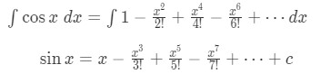
Equation 6: Taylor Expansion Relationship cosx and sinx pt.2 See that if \(x=0\), then
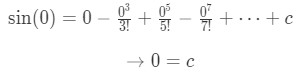
Equation 6: Taylor Expansion Relationship cosx and sinx pt.3 So the integral of cosine is
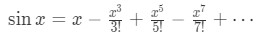
Equation 6: Taylor Expansion Relationship cosx and sinx pt.4 which is the Taylor Expansion of \(\sin x\). Likewise, the integral of \(\sin x\) gives:
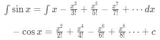
Equation 6: Taylor Expansion Relationship cosx and sinx pt.5 See if \(x=0\), then,
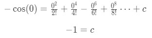
Equation 6: Taylor Expansion Relationship cosx and sinx pt.6 Then we are left with:
Equation 6: Taylor Expansion Relationship cosx and sinx pt.7 Dividing both sides of the equation by -1 gives:
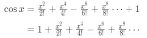
Equation 6: Taylor Expansion Relationship cosx and sinx pt.8 which is the Taylor Expansion of \(\cos x\).
Now that we know how to use the Taylor Series Formula, let's learn how to manipulate the formula to find Taylor Series of harder functions.
Question 6:Find the Taylor Series of \(f(x) = \frac{\sin x}{x}\).
- So we see that the function has \(\sin x\) in it. We know that \(\sin x\) has the common Taylor series:
Equation 7: Taylor Series of sinx/x pt.1 So if we were to divide both sides by \(x\), then we will get:
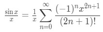
Equation 7: Taylor Series of sinx/x pt.2 We can manipulate the right hand side so that:
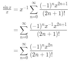
Equation 7: Taylor Series of sinx/x pt.3 and so we just found the Taylor series for \(\frac{\sin x}{x}\). Let's do a harder question.
Question 7: Find the Taylor Series of
-
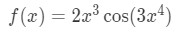
Equation 8: Taylor Series of 2x^3cos(3x^4) pt.1 Notice that cosine is in the function. So we probably want to use the Taylor Series:
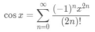
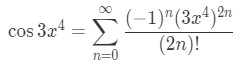
Equation 8: Taylor Series of 2x^3cos(3x^4) pt.2 See that inside the cosine is \(3x^{4}\). So what were going to do is replace all the \(x\)'s, and make them into \(3x^{4}\). In other words,

Equation 8: Taylor Series of 2x^3cos(3x^4) pt.3 Doing so gives us:
Equation 8: Taylor Series of 2x^3cos(3x^4) pt.4 Now we are going to multiply both sides of the equation by \(2x^{3}\). This leads to:
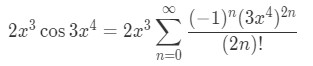
Equation 8: Taylor Series of 2x^3cos(3x^4) pt.5 Now we are going to clean up the series a little bit so that everything is inside the general term.
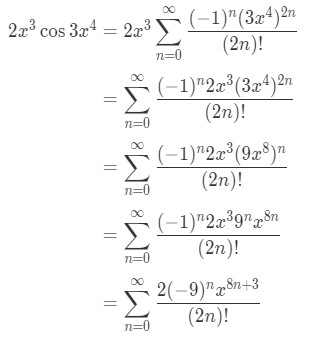
Equation 8: Taylor Series of 2x^3cos(3x^4) pt.6
Thus we are done and this is the Taylor Series of \(2x^{3} \cos (3x^{4})\). If you want to do more practice problems, then I suggest you look at this link.
http://tutorial.math.lamar.edu/Problems/CalcII/TaylorSeries.aspxEach question has a step-by-step solution, so you can check your work!
Note that the Taylor Series Expansion goes on as \(n \)→\( \infty\), but in practicality we cannot go to infinity. As humans (or even computers) we cannot go on forever, so we have to stop somewhere. This means we need to alter the formula for us so that it is computable.
We alter the formula will be:

Notice that since we stopped looking for terms after n, we have to make it an approximation instead. This formula is known as the Taylor approximation. It is a well known formula that is used to approximate certain values.
Notice on the right hand side of the equation that it is a polynomial of degree n. We actually call this the Taylor polynomial \(T_{n} (x)\). In other words, the Taylor polynomial formula is:

Let's do an example of finding the Taylor polynomial, and approximating a value.
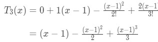
Question 8: Find the \(3^{rd}\) degree Taylor Polynomial of \(f(x) = \ln (x)\) centred at \(a = 1\). Then approximate \(\ln (2)\).
- If we are doing a Taylor Polynomial of degree 3 centred at \(a = 1\), then use the formula up to the \(4^{th}\) term:

Equation 9: Taylor Series Polynomial lnx pt.1 Notice that taking the derivatives gives us:
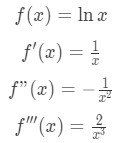
Equation 9: Taylor Series Polynomial lnx pt.2 We also know that \(a = 1\), so:
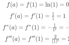
Equation 9: Taylor Series Polynomial lnx pt.3 Just in case you forgot, \(\ln 1\) gives us 0. That's why \(f(a) = 0\). Now plugging everything into the formula of the \(3^{rd}\) degree Taylor polynomial gives:
Equation 9: Taylor Series Polynomial lnx pt.4 Now we have to approximate \(\ln (2)\). In order to do this, we need to use the Taylor polynomial that we just found. Notice that according to the Taylor approximation:

Equation 9: Taylor Series Polynomial lnx pt.5 This means that:
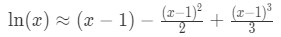
Equation 9: Taylor Series Polynomial lnx pt.6 If we are to set \(x = 2\), then we will see that:
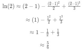
Equation 9: Taylor Series Polynomial lnx pt.7 So \(\ln (2)\) is approximately around \(\frac{5}{6}\). See that \(\frac{5}{6}\) in decimal form is 0.833333...
Now if you pull out your calculator, we are actually pretty close. The actual value of \(\ln (2)\) is 0.69314718056....
We know that Taylor Approximation is just an approximation. However, what if we want to know the difference between the actual value and the approximated value? We call the difference the error term, and it can be calculated using the following formula:
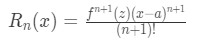
Keep in mind that the \(z\) variable is a value that is between \(a\) and \(x\), which gives the largest possible error.
Let's use the error term formula to find the error of our previous question.
Question 9: Find the error of \(\ln (2)\).
- In order to find the error, we need to find

Equation 10: Taylor Series Error term ln(2) pt.1 Notice from our previous question that we found the Taylor polynomial of degree 3. So we set \(n = 3\). This means we need to find:

Equation 10: Taylor Series Error term ln(2) pt.2 See that the fourth derivative of the function is:

Equation 10: Taylor Series Error term ln(2) pt.3 Now our function is in terms of \(x\), but we need it in term of \(z\). So we just set \(z = x\). This means that:
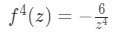
Equation 10: Taylor Series Error term ln(2) pt.4 So plugging this into our error term formula gives us:
Equation 10: Taylor Series Error term ln(2) pt.5 Remember that we set \(x=2\) and \(a=1\), so we have:
Equation 10: Taylor Series Error term ln(2) pt.6 Since we are talking the error of our approximation, the negative sign doesn't matter here. So realistically we are looking at:
Equation 10: Taylor Series Error term ln(2) pt.7 Now recall that \(z\) is a number between \(a\) and \(x\) which makes the error term the largest value. In other words, \(z\) must be:

Equation 10: Taylor Series Error term ln(2) pt.8 because \(a=1\), and \(x=2\). Now what \(z\) value must we pick so that our error term is the largest?
Notice that the variable \(z\) is in the denominator. So if we pick smaller values of \(z\), then the error term will become bigger. Since the smallest value of \(z\) we can pick is 1, then we set \(z = 1\). Thus,
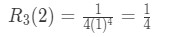
Equation 10: Taylor Series Error term ln(2) pt.9 is our error.
Now think of it like this. If we were to add the error term and the approximated value together, wouldn't I get the actual value? This is correct! In fact, we can say this formally. If the Taylor polynomial is the approximated function and \(R_{n} (x)\) is the error term, then adding them gives the actual function. In other words,

This is known as Taylor Theorem.