Overview
Watch
Read
Next Steps
Read
Mastering Slope and Equation of Tangent Lines in Calculus
The derivative of a function is interpreted as the slope of the tangent line to the curve of the function at a certain given point. In this section, we will explore the meaning of a derivative of a function, as well as learning how to find the slope-point form of the equation of a tangent line, as well as normal lines, to a curve at multiple given points.
Understanding the slope of tangent lines and their equations is crucial in calculus. The introduction video provides a solid foundation for grasping these concepts. Remember that the slope of a tangent line at a point is equivalent to the derivative of the function at that point. This relationship is fundamental in finding equations of tangent lines. To master these skills, practice solving problems involving different functions. Start with simple polynomials and progress to more complex functions. Don't hesitate to revisit the video for clarification on challenging aspects. Explore additional resources, such as online tutorials and textbooks, to deepen your understanding. The ability to find slopes and equations of tangent lines is essential for many advanced calculus topics, including optimization and related rates. By mastering these concepts, you'll be well-prepared for future mathematical challenges. Keep practicing and stay curious about the fascinating world of calculus!
Example:
Connecting: Derivative & Slope & Equation of Tangent Line
Exercise: The graph of the quadratic function \(f\left( x \right) = \frac{1}{2}{x^2} + 2x - 1\) is shown below.
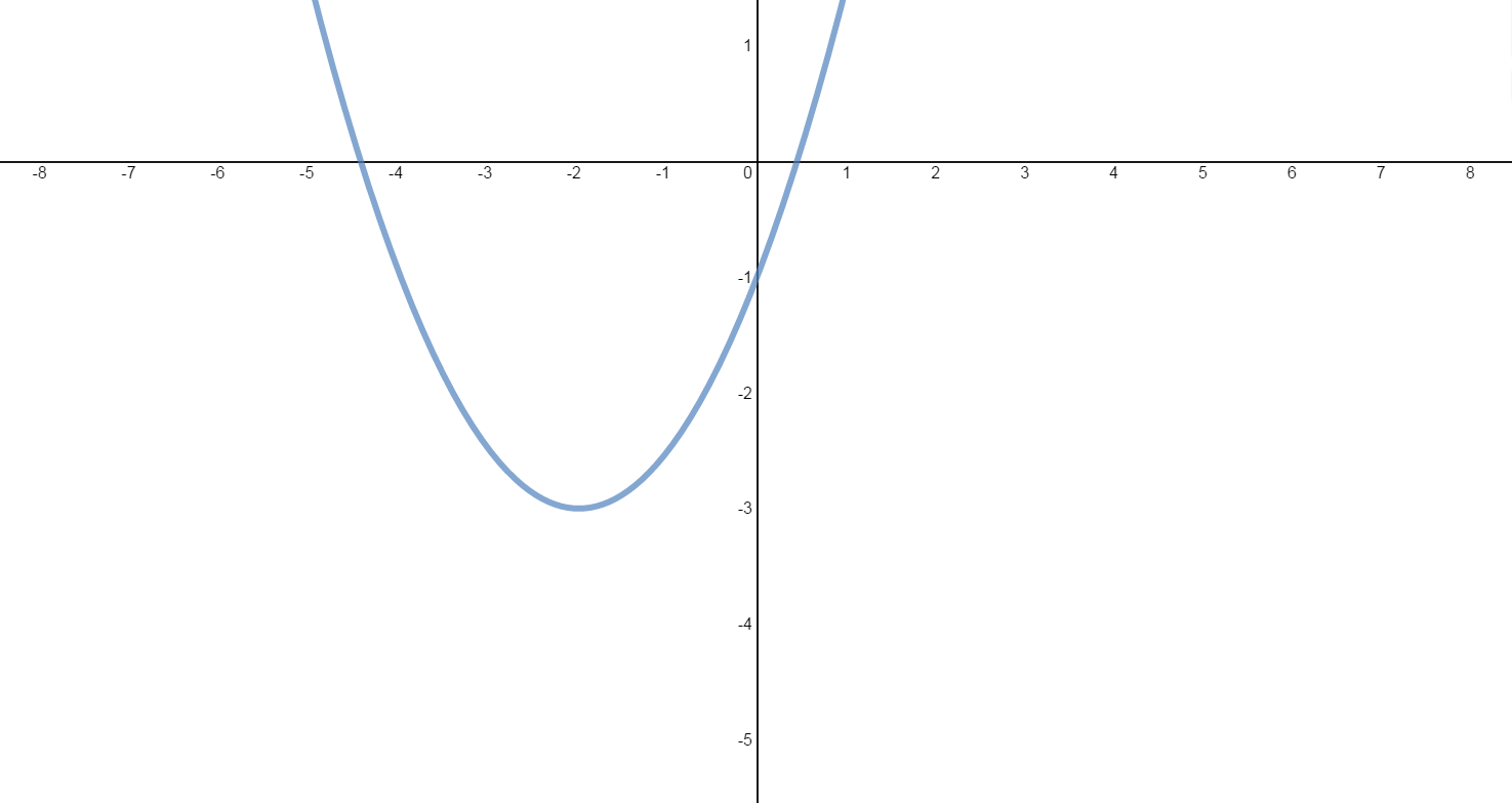 Find and interpret \(f'\left( x \right)\).
Step 1: Understanding the Problem
In this exercise, we are given a quadratic function \(f(x) = \frac{1}{2}x^2 + 2x - 1\). Our task is to find the derivative of this function, denoted as \(f'(x)\), and interpret its meaning. The derivative of a function at a given point provides the slope of the tangent line to the graph of the function at that point.
Step 2: Applying the Power Rule
Since we are dealing with a polynomial, we can use the power rule to find the derivative of each term in the polynomial. The power rule states that if \(f(x) = ax^n\), then \(f'(x) = anx^{n-1}\).
Let's start with the first term, \(\frac{1}{2}x^2\):
- Bring the exponent 2 to the front and multiply it by \(\frac{1}{2}\), giving us \(1x\).
- Subtract 1 from the exponent, resulting in \(x^1\) or simply \(x\).
Next, consider the second term, \(2x\):
- We can write this as \(2x^1\).
- Bring the exponent 1 to the front and multiply it by 2, giving us \(2\).
- Subtract 1 from the exponent, resulting in \(x^0\), which is 1.
Finally, the last term is a constant, \(-1\):
- The derivative of any constant is 0.
Step 3: Combining the Derivatives
Now, we combine the derivatives of each term to get the overall derivative of the function:
- The derivative of \(\frac{1}{2}x^2\) is \(x\).
- The derivative of \(2x\) is \(2\).
- The derivative of \(-1\) is \(0\).
Step 4: Interpreting the Derivative
The derivative \(f'(x) = x + 2\) represents the slope of the tangent line to the graph of the function at any point \(x\). To understand this better, let's consider a specific point on the graph.
For example, if we pick the point where \(x = -6\):
- We substitute \(-6\) into the derivative equation: \(f'(-6) = -6 + 2 = -4\).
- This means that the slope of the tangent line to the graph at \(x = -6\) is \(-4\).
The negative slope indicates that the tangent line is decreasing at this point, similar to driving downhill. Conversely, a positive slope would indicate an increasing tangent line, similar to driving uphill.
Step 5: General Interpretation
In general, for any function \(y = f(x)\), the derivative \(f'(x)\) can be interpreted geometrically as the slope of the tangent line to the graph of the function at the point \((x, f(x))\). This means that \(f'(x)\) gives us the rate of change of the function at any given point \(x\).
FAQs
Here are some frequently asked questions about slope and equation of tangent lines:
1. How do you find the slope of a tangent line?
To find the slope of a tangent line at a specific point, you need to calculate the derivative of the function and evaluate it at that point. The derivative gives the instantaneous rate of change, which is equivalent to the slope of the tangent line.
2. What is the formula for the slope of a line in tan?
The formula for the slope of a tangent line is m = f'(x), where f'(x) is the derivative of the function f(x) evaluated at the point of tangency.
3. What is the equation for tangent in slope form?
The equation of a tangent line in slope form is y - y1 = m(x - x1), where (x1, y1) is the point of tangency and m is the slope of the tangent line.
4. Why is the derivative the slope of the tangent?
The derivative represents the instantaneous rate of change of a function at a given point. Geometrically, this rate of change corresponds to the slope of the line tangent to the function's graph at that point.
5. How do you write the equation of the tangent line?
To write the equation of a tangent line: 1) Find the derivative of the function. 2) Evaluate the derivative at the point of tangency to get the slope. 3) Use the point-slope form y - y1 = m(x - x1) with the point of tangency and calculated slope. 4) Simplify to get the final equation.
Prerequisite Topics
Understanding the slope and equation of a tangent line is a crucial concept in calculus and advanced mathematics. However, to fully grasp this topic, it's essential to have a solid foundation in several prerequisite areas. Let's explore how these fundamental concepts contribute to your understanding of tangent lines and their equations.
First and foremost, the concept of rate of change is integral to understanding slopes and tangent lines. In calculus, the tangent line represents the instantaneous rate of change of a function at a specific point. This connection between rate of change and tangent lines is particularly relevant when studying derivatives and their applications in various fields, including economics.
Another crucial prerequisite is the power of a power rule. This algebraic concept becomes especially important when dealing with the power rule for derivatives, which is frequently used in finding the equations of tangent lines for polynomial functions.
A strong grasp of graphing linear functions using a single point and slope is essential. This skill directly translates to working with tangent lines, as a tangent line is essentially a linear function that touches a curve at a single point. Understanding how to graph a line given a point and its slope is crucial for visualizing and constructing tangent lines.
Similarly, familiarity with graphing from slope-intercept form y=mx+b is valuable. This knowledge extends to the point-slope form of a line, which is often used when working with tangent lines. Being able to convert between different forms of linear equations enhances your ability to work with tangent line equations efficiently.
An understanding of special cases of linear equations, such as horizontal lines, is also beneficial. In the context of tangent lines, horizontal tangent lines occur at local maximum or minimum points of a function, making this knowledge particularly relevant in optimization problems.
Lastly, being familiar with the applications of polynomial functions provides real-world context for tangent lines. Many practical problems involve finding tangent lines to polynomial curves, and understanding these applications can make the concept more meaningful and relevant.
By mastering these prerequisite topics, you'll build a strong foundation for understanding the slope and equation of tangent lines. This knowledge will not only help you in your current studies but also prepare you for more advanced mathematical concepts in calculus and beyond.