Equation of the best fit line

All You Need in One Place

Everything you need for better marks in primary, GCSE, and A-level classes.

Learn with Confidence

We’ve mastered the UK’s national curriculum so you can study with confidence.

Instant and Unlimited Help

24/7 access to the best tips, walkthroughs, and practice questions.

0/1
?
Intros
Lessons

  1. • Formula for the Best Fit Line
    • What are Residuals?
0/5
?
Examples
Lessons
  1. Determining the Equation for a Best Fit Line
    Given the following bivariate data give the equation for the best fit line and plot it on the given graph.

    x

    y

    1

    2

    2

    2

    3

    4

    4

    5


    Plot the best fit line
    1. Determining the Equation for a Best Fit Line using Calculator Commands
      For the following bivariate data:

      x

      y

      1

      9

      2

      7

      3

      8

      4

      5

      5

      5

      6

      3

      7

      2


      1. Using a graphing calculator plot the points on a graph
      2. Still using your graphing calculator find the equation for the best fit line and plot it on the same graph
    2. Interpretation graphical Data
      In Skyrim (a video game) I plotted what level I was when I killed my first 5 dragons. The graphical data is given below:

      # of dragons killed

      Corresponding level

      1

      Level 4

      2

      Level 5

      3

      Level 6

      4

      Level 6

      5

      Level 7


      Equation of the best fit line
      1. What is the sum of all the residuals squared?
      2. Using the data above extrapolate what my level will be when I kill my 8th dragon. Is this a good estimation? Why or why not?
    Topic Notes
    ?
    Table of Contents:

    Equation of the best fit line


    This lesson is a continuation of our past two lessons, where we talked about bivariate data, scatter plots and correlation, and then learnt about regression analysis. Therefore, we will be using the concepts we acquired throughout those two lessons and construct on them to study the line of best fit definition and characteristics.

    What is a line of best fit


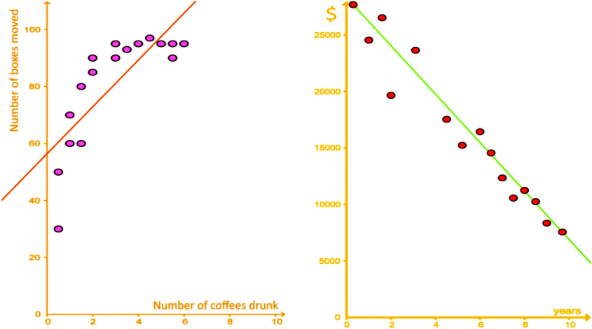
    As we saw in our past lesson, a line of best fit (or best fit line) is simply straight line that tries to represent the data points in a scatter plot as best as possible. This doesnt mean that this line will touch every single point from the data in the plot, actually a line of best fit may touch a few, all or NONE of the data points plotted in the graph. For that reason, the line of best fit is also called the trend line because instead of exactly representing each single point of the data set, it does all it can by presenting the overall trend that the data points follow, it provides a view of the behaviour of the data points and how the variables are correlated with each other.

    Equation of the best fit line
    Figure 1: Examples of lines of best fit in bivariate data scatter plots


    How to find line of best fit


    Since the line of best fit is simply a straight line, it can be mathematically defined through the equation for a straight line:

    y=mx+b  y=mx+b \;   y=ax+b \; y=ax+b
    Equation 1: Equation for the best fit line (equation for a straight line)

    Where we know that:
    y=y = dependent variable
    x=x = independent variable
    m=a=m=a = slope of the line (the name can be different depending on the textbook you are using)
    b=yb=y-intercept (point in the graph where the line crosses the yy axis

    Notice the slope can have either one of two names: mm or aa, the name differs depending on which textbook you are using in your class or to study; for this lesson, we will keep the name aa, just remember that we are talking about the slope of best fit line.

    For the cases in which we are looking at a linear regression analysis graph where a bivariate set of data has been plotted, we will always have the values of the variables xix_i and yiy_i (since these are the values given in the bivariate data set) and so, we will usually have to solve for the slope and the y-intercept from the equation for the line of best fit.

    In other words, when having a bivariate data set, xix_i and yiy_i are provided, so a and b have to be calculated (this is not always the case, the line of best fit equation can be used to solve for the values of the variables themselves when given the slope of the line and the y-intercept, but if the data table is provided, then we will be solving for aa and bb).

    Equation of the best fit line
    Figure 2: Example of Bivariate set of data in a scatter plot

    The formulas for the slope and the y-intercept are as follows:

    a=ni=1nxiyi    i=1nxii=1nyini=1nxi2    (i=1nxi)2 \large a = \frac{n \sum_{i=1}^{n}x_iy_i \;- \; \sum_{i=1}^{n}x_i \sum_{i=1}^{n}y_i}{n \sum_{i=1}^{n}x_i^2 \; - \; (\sum_{i=1}^{n}x_i)^2} \quad and=b=yax \enspace = b = \overline{y} - a\overline{x}
    Equation 2: formulas for slope and y-intercept

    Where:
    n=n= number of data points
    yi=y_i=dependent variable data value
    xi=x_i= independent variable data value
    a=a= slope of the best fit line
    b=yb=y -intercept
    x\overline{x}= mean for the sample of xx values
    y \overline{y} = mean for the sample of yy values
    i=1n \sum_{i=1}^{n} is the symbol for summation
    therefore: i=1nxi=x1  +  x2  +...+xn\large \sum_{i=1}^{n}x_i = x_1 \;+\; x_2 \; + \, ... \, + \, x_n

    In equation 2, notice that b is defined in terms of a, therefore, you will always solve for a first; b is also defined in terms of the means x\overline{x} and y\overline{y}, which takes us to an important realization: the data points in the set shown in a regression analysis scatter plot count as a sample, not as a whole population. If you think about it, this makes sense, since a regression analysis scatter plot is usually used to find missing points that have not been graphed, but can be inferred by the relationship shown throughout the given data points.
    Therefore, when obtaining the mean of the values for each of the variables used in the analysis, we are taking the mean of sample data points and so the notation for the mean of a sample: x\overline{x}.

    After solving aa and bb, we can use these values to solve the best fit line equation as shown in equation 1, and plot the best fit line graph in the scatter plot.

    How to draw a line of best fit


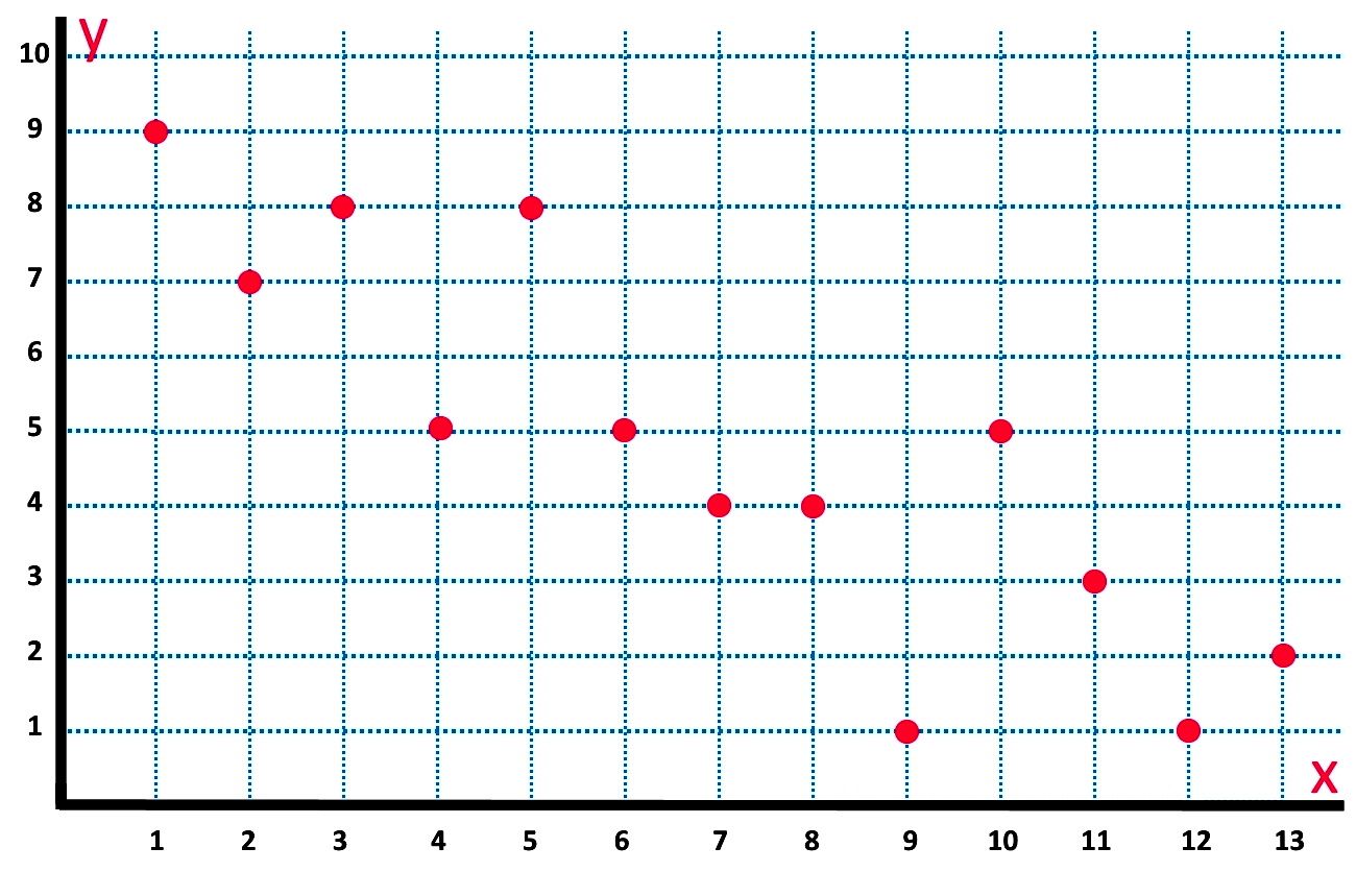
    Let us use the method described above to obtain the best fit line of the bivariate data scatter plot shown in figure 2. We start by producing its corresponding data table so we know the values of xix_i and yiy_i .

    Equation of the best fit line
    Figure 3: Data table for bivariate data set in figure 2

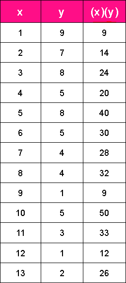
    So let us solve for a by making the calculations in pieces:

    a=ni=1nxiyi    i=1nxii=1nyini=1nxi2    (i=1nxi)2 \large a = \frac{n \sum_{i=1}^{n}x_iy_i \;- \; \sum_{i=1}^{n}x_i \sum_{i=1}^{n}y_i}{n \sum_{i=1}^{n}x_i^2 \; - \; (\sum_{i=1}^{n}x_i)^2}

    where:n=13 n =13

    i=113xiyi=x1y1  +  x2y2  +...+x13y13 \large \sum_{i=1}^{13}x_iy_i = x_1y_1 \;+\; x_2y_2 \; + \, ... \, + \, x_{13}y_{13}=9+14+24+20+40+30+28+32+9+50+33+12+26=327 = 9+14+24+20+40+30+28+32+9+50+33+12+26=327

    i=113xi=x1  +  x2  +...+x13\large \sum_{i=1}^{13}x_i= x_1 \;+\; x_2 \; + \, ... \, + \, x_{13} =1+2+3+4+5+6+7+8+9+10+11+12+13=91= 1+2+3+4+5+6+7+8+9+10+11+12+13=91

    i=113yi=y1  +  y2  +...+y13\large \sum_{i=1}^{13}y_i= y_1 \;+\; y_2 \; + \, ... \, + \, y_{13} =9+7+8+5+8+5+4+4+1+5+3+1+2=62= 9+7+8+5+8+5+4+4+1+5+3+1+2=62

    i=113xi2\large \sum_{i=1}^{13}x_i^2 =1+4+9+16+25+36+49+64+81+100+121+144+169=819= 1+4+9+16+25+36+49+64+81+100+121+144+169=819

    (i=113xi)2 \large (\sum_{i=1}^{13}x_i)^2 =(91)2=8,281=(91)^{2}=8,281

    therefore:

    a=13(327)(91)(62)13(819)8,281=4,2515,64210,6478,281=1,3912,366=0.59\large a = \frac{13(327)-(91)(62)}{13(819)-8,281} = \frac{4,251-5,642}{10,647-8,281} = \frac{-1,391}{2,366} = - 0.59
    Equation 3: Solving for the slope of the best fit line

    Now we solve for b:

    b=yaxb = \overline{y}- a\overline{x}

    where:

    x=1+2+3+4+5+6+7+8+9+10+11+12+1313=9113=7\overline{x}= \frac{1+2+3+4+5+6+7+8+9+10+11+12+13}{13} = \frac{91}{13} =7

    y=9+7+8+5+8+5+4+4+1+5+3+1+213=6213=4.77\overline{y}= \frac{9+7+8+5+8+5+4+4+1+5+3+1+2}{13} = \frac{62}{13} =4.77

    therefore:  b=4.77(0.59)(7)=4.77+4.13=8.9\; b =4.77 - (-0.59)(7) = 4.77 + 4.13 = 8.9
    Equation 4: Solving for the y-intercept

    And so, we can obtain the points for our trend line using the line of best fit formula from equation 1:

    y=ax+by = ax +b

    whenx=0 \,x = 0 \, y=0+8.9=8.9 \, y = 0 +8.9 = 8.9

    whenx=13 \,x = 13 \, y=(0.59)(13)+8.9=7.67+8.9=1.23 \, y = (-0.59)(13) +8.9 = -7.67 + 8.9 = 1.23
    Equation 5: Obtaining two points for the line of best fit

    And now we can graph the two points found above: (0, 8.9) and (13, 1.23); we connect them with a straight line and we find the line of best fit!

    Equation of the best fit line
    Figure 4: Plotting the best fit line

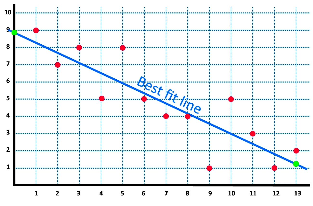
    And so, for the scatter plot of the line of best fit as seen in figure 4, we can see that the points (0, 8.9) and (13, 1.23) are shown in green, and the best fit line is shown in blue.

    Let us work through another example so you can get more practice:

    Example 1

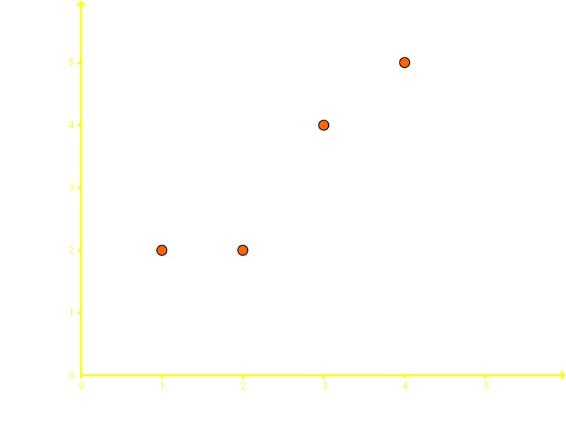
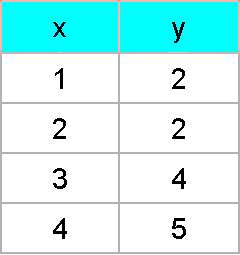
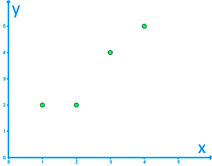
    Given the following bivariate data, what is the line of best fit?
    Use the the equation for the line of best fit and plot it in the diagram provided.

    Equation of the best fit line
    Figure 5: Data table for bivariate data set


    Equation of the best fit line
    Figure 6: Bivariate set of data in a scatter plot

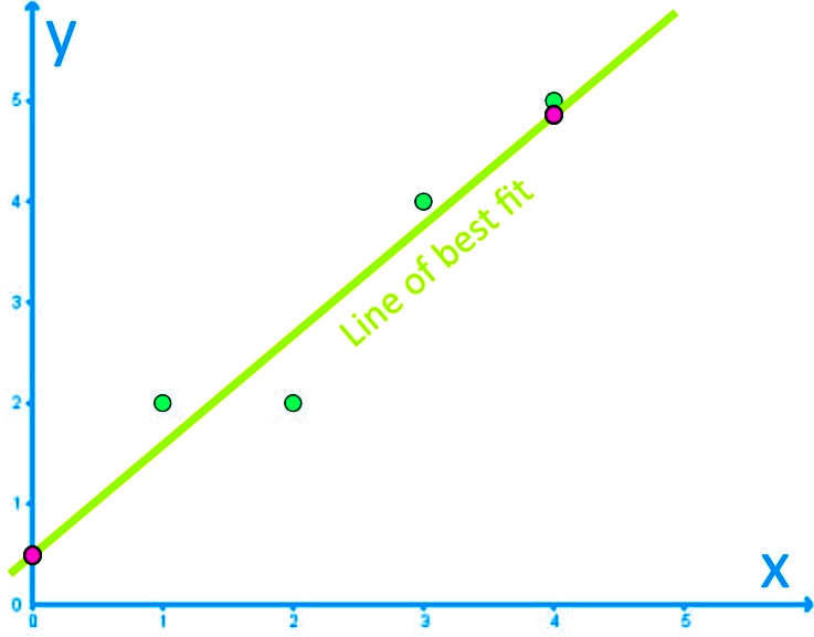
    We start by doing the calculation for the slope of the line of best fit:

    a=ni=1nxiyi    i=1nxii=1nyini=1nxi2    (i=1nxi)2 \large a = \frac{n \sum_{i=1}^{n}x_iy_i \;- \; \sum_{i=1}^{n}x_i \sum_{i=1}^{n}y_i}{n \sum_{i=1}^{n}x_i^2 \; - \; (\sum_{i=1}^{n}x_i)^2}

    where:n=13 n =13

    i=14xiyi=x1y1  +  x2y2  +x3y3+x4y4 \large \sum_{i=1}^{4}x_iy_i = x_1y_1 \;+\; x_2y_2 \; + \, x_3y_3 \, + \, x_{4}y_{4}=(1)(2)+(2)(2)+(3)(4)+(4)(5)=38 =(1)(2)+(2)(2)+(3)(4)+(4)(5)=38

    i=14xi=x1  +  x2  +x3+x4\large \sum_{i=1}^{4}x_i = x_1 \;+\; x_2 \; + \, x_3 \, + \, x_{4}=1+2+3+4=10 =1+2+3+4=10

    i=14yi=y1  +  y2  +y3+y4 \large \sum_{i=1}^{4}y_i = y_1 \;+\; y_2 \; + \, y_3 \, + \, y_{4}=2+2+4+5=13 =2+2+4+5=13

    i=14xi2 \large \sum_{i=1}^{4}x_i^2 =1+4+9+16=30= 1+4+9+16=30

    (i=14xi)2 \large (\sum_{i=1}^{4}x_i)^2 =(10)2=100=(10)^{2}=100

    therefore:

    a=4(38)(10)(13)4(30)100=152130120100=2220=1.1\large a = \frac{4(38)-(10)(13)}{4(30)-100} = \frac{152-130}{120-100} = \frac{22}{20} = 1.1
    Equation 6: Solving for the slope of the best fit line

    Now we solve for b:

    b=yaxb = \overline{y}- a\overline{x}

    where:

    x=1+2+3+44=104=2.5 \overline{x}= \frac{1+2+3+4}{4} = \frac{10}{4} =2.5

    y=2+2+4+54=134=3.25 \overline{y}= \frac{2+2+4+5}{4} = \frac{13}{4} =3.25

    therefore:  b=3.25(1.1)(2.5)=3.252.75=0.5\; b =3.25 - (1.1)(2.5) = 3.25 - 2.75 = 0.5
    Equation 7: Solving for the y-intercept

    And so, we can obtain the points for our trend line using the line of best fit formula from equation 1:

    y=ax+by = ax +b

    whenx=0 \,x = 0 \, y=0+0.5=0.5 \, y = 0 +0.5 = 0.5

    whenx=4 \,x = 4 \, y=(1.1)(4)+0.5=4.4+0.5=4.9 \, y = (1.1)(4) +0.5 = 4.4 + 0.5 = 4.9
    Equation 8: Obtaining two points for the line of best fit

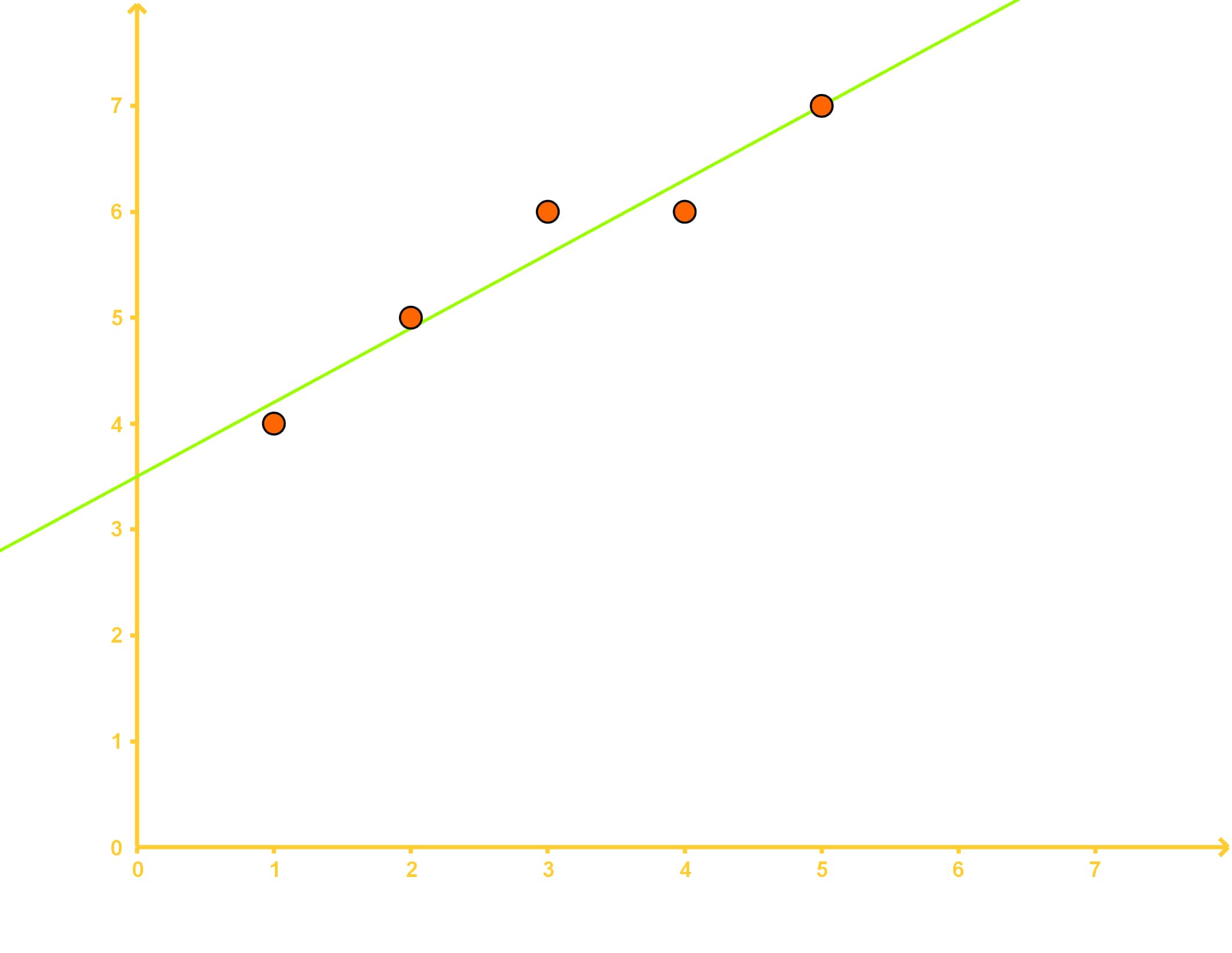
    And now we can graph the two points found above: (0, 0.5) and (4, 4.9); we connect them with a straight line and we obtain the line of best fit:

    Equation of the best fit line
    Figure 7: Plotting the best fit line

    No we end this lesson with a few recommendations: this lesson on the equation of the line of best fit provides many more examples that you can work through so you continue practice what you learned today. And for even more practice on you own, this lines of best fit worksheet can be printed out and worked through!

    This is it for our lesson of today, see you in the next one!
    The best fit line has the equation: y=ax+by=ax+b, where aa and bb are given as:
    a=nxyxynx2(x)2a=\frac{n\sum xy-\sum x \sum y}{n\sum x^2-(\sum x)^2}
    b=yaxb=\overline{y}-a\overline{x}