Transforming shapes with matrices

Get the most by viewing this topic in your current grade. Pick your course now.

?
Intros
Lessons
  1. Transforming shapes with matrices overview
?
Examples
Lessons
  1. Finding the Transformed Polygons
    Apply the transformation matrix TT to the following vertices to find the transformed vertices:
    1. Transforming shapes with matrices
    2. Transforming shapes with matrices
    3. Transforming shapes with matrices
  2. Graphing the Transformed Polygon
    Plot the vertices Transforming shapes with matrices on the graph. Then apply the transformation matrix Transforming shapes with matrices, to the vertices to find the transformed polygon, and then plot the transformed polygon on the graph.
    1. Plot the vertices Transforming shapes with matrices on the graph. Then apply the transformation matrix Transforming shapes with matrices, to the vertices to find the transformed polygon, and then plot the transformed polygon on the graph.
      1. Plot the vertices Transforming shapes with matrices on the graph. Then apply the transformation matrix Transforming shapes with matrices, to the vertices to find the transformed polygon, and then plot the transformed polygon on the graph.
        Topic Notes
        ?
        In this section, we will learn how to transform shapes with matrices. Instead of one column vector, we are going to have multiple vertices which create a shape. What we can do to this shape is use the transformation matrix to change the length and size of that shape. To do this computation, we merge all the vertices into one matrix and then multiply it with the transformation matrix. Doing so will give us another matrix. We will then take a look at each transformed vertices separately in the matrix to see the new transformed shape. Note that transforming the shape does not change the number of sides. We will take a look at some questions which involve transforming shapes, and then graph them to notice the changes between the normal shape and the transformed shape.

        Introduction: Transforming Shapes with Matrices

        Transforming shapes with matrices is a powerful concept in computer graphics and linear algebra. Building upon the foundation of transforming individual vectors, this technique extends to manipulating entire shapes. The process involves applying transformation matrices to the vertices of a shape, effectively altering its position, size, or orientation in space. Our introduction video serves as a crucial starting point, offering a visual and intuitive explanation of this complex topic. It demonstrates how matrices can be used to rotate, scale, or translate shapes with precision and efficiency. By understanding this concept, you'll gain insight into how 3D graphics engines and animation software manipulate objects. The transformation of shapes using matrices is not only mathematically elegant but also practical, forming the backbone of numerous applications in computer graphics, game development, and digital animation. This fundamental principle opens up a world of possibilities for creating dynamic and interactive visual experiences.

        Understanding Shapes as Collections of Vertices

        In the world of computer graphics and geometry, shapes are often represented as collections of vertices. This fundamental concept is crucial for understanding how objects are defined and manipulated in digital environments. Let's explore this idea using the simple example of a square, which will help us grasp how vertices and vectors work together to create shapes.

        A square is a basic polygon with four equal sides and four right angles. In terms of vertices, a square is composed of four distinct points, each representing a corner of the shape. These vertices are the building blocks that define the square's structure and position in space.

        Each vertex of a square is represented as a vector, which is essentially a mathematical entity that has both magnitude and direction. In a two-dimensional space, a vector typically consists of two components: an x-coordinate and a y-coordinate. These coordinates pinpoint the exact location of each vertex relative to a defined origin point.

        Let's visualize a square with labeled vertices:

            A (0,1) -------- B (1,1)
            |                |
            |                |
            |                |
            |                |
            C (0,0) -------- D (1,0)
            

        In this representation:

        • Vertex A is at coordinates (0,1)
        • Vertex B is at coordinates (1,1)
        • Vertex C is at coordinates (0,0)
        • Vertex D is at coordinates (1,0)

        Each of these vertices is a vector that defines a specific point in the 2D plane. By connecting these vertices in the correct order (A to B, B to D, D to C, and C back to A), we create the shape of a square.

        It's important to note that this concept of representing shapes as collections of vertices extends far beyond just squares. This principle applies to all polygons and even three-dimensional objects. For instance:

        • A triangle would be represented by three vertices
        • A pentagon would have five vertices
        • A cube in 3D space would be defined by eight vertices

        The power of this representation lies in its versatility and efficiency. By manipulating the vectors that represent these vertices, we can easily transform shapes in various ways:

        • Translation: Moving the entire shape by adjusting all vertex coordinates
        • Rotation: Changing the orientation of the shape by rotating the vertices around a point
        • Scaling: Enlarging or shrinking the shape by multiplying vertex coordinates

        In computer graphics and 3D modeling, more complex shapes and objects are created by combining multiple polygons, each defined by its own set of vertices. This approach allows for the creation of intricate models and scenes, all built upon the fundamental concept of vertices as vector representations.

        Understanding shapes as collections of vertices is not just a theoretical concept; it has practical applications in various fields:

        • Video game development: Creating and manipulating game objects
        • Computer-aided design (CAD): Designing precise 2D and 3D models
        • Computer vision: Analyzing and processing visual data
        • Geographic Information Systems (GIS): Representing geographical features

        By grasping this fundamental principle of representing shapes through vertices and vectors, you gain insight into how digital graphics and geometric computations work at their core. This knowledge forms the basis for more advanced concepts in computer graphics, mathematics, and related fields, opening up a world of possibilities in digital design and analysis.

        Creating a Matrix from Shape Vertices

        In computer graphics and 3D modeling, combining individual vertex vectors into a single matrix is a crucial step in the process of transforming shapes. This technique, known as matrix representation of vertices, allows for efficient manipulation and transformation of geometric objects. Understanding this process is essential for anyone working with computer graphics, game development, or 3D modeling software.

        The process of combining vertex vectors into a matrix begins with identifying the individual vertices that make up a shape. Each vertex is represented by a vector, typically containing its x, y, and z coordinates in 3D space (or x and y for 2D shapes). These individual vectors are then combined into a single matrix, where each column represents a vertex of the shape.

        This step is necessary for transforming shapes because it allows for the application of matrix operations to all vertices simultaneously. By representing the shape's vertices as a matrix, we can perform various transformations such as translation, rotation, and scaling using matrix multiplication. This approach is far more efficient than applying transformations to each vertex individually, especially for complex shapes with numerous vertices.

        Let's consider a simple example of how a square's four vertices are combined into a 2x4 matrix. Imagine a square with vertices at (0,0), (1,0), (1,1), and (0,1) in a 2D coordinate system. The matrix representation would look like this:

        [0 1 1 0]
        [0 0 1 1]

        In this matrix, each column represents a vertex of the square. The first row contains the x-coordinates of all vertices, while the second row contains the y-coordinates. This compact representation allows us to apply transformations to the entire shape by performing matrix operations on this single matrix.

        The concept of combining vertices into a matrix scales seamlessly to other shapes with more vertices. For instance, a cube in 3D space would have eight vertices, resulting in a 3x8 matrix (three rows for x, y, and z coordinates, and eight columns for each vertex). More complex shapes like spheres or detailed 3D models can have hundreds or thousands of vertices, all represented in a single matrix.

        As the number of vertices increases, the benefits of this matrix representation become even more apparent. Transforming a shape with thousands of vertices becomes a simple matter of matrix multiplication, rather than iterating through each vertex individually. This efficiency is crucial in real-time graphics applications, such as video games or interactive 3D visualizations, where performance is paramount.

        Moreover, this matrix representation facilitates more advanced operations in computer graphics. For example, it enables the application of complex transformations like perspective projection, which is essential for rendering 3D scenes on 2D displays. It also simplifies the process of applying multiple transformations in sequence, as these can be combined into a single transformation matrix and then applied to the vertex matrix in one operation.

        In conclusion, the process of combining individual vertex vectors into a single matrix is a fundamental technique in computer graphics and 3D modeling. It provides an efficient and versatile way to represent and transform shapes, regardless of their complexity. By understanding this concept, developers and designers can create more efficient and powerful graphics applications, paving the way for more immersive and visually stunning digital experiences.

        Applying the Transformation Matrix

        The process of multiplying a transformation matrix with a shape's vertex matrix is a fundamental operation in computer graphics and 3D modeling. This technique allows us to transform entire shapes or objects in a single operation, rather than transforming individual vectors one at a time. Understanding this process is crucial for anyone working with 3D graphics or geometric transformations.

        To begin, let's consider the difference between transforming a single vector and transforming an entire shape. When we transform a single vector, we multiply the transformation matrix by a single column vector representing the point's coordinates. However, when transforming a shape, we multiply the transformation matrix by a matrix containing all the vertices of the shape.

        The step-by-step process of multiplying a transformation matrix with a shape's vertex matrix is as follows:

        1. Prepare the transformation matrix: This is typically a 4x4 matrix for 3D transformations or a 3x3 matrix for 2D transformations.
        2. Create the vertex matrix: Arrange all the vertices of the shape into a matrix, where each column represents a vertex.
        3. Perform matrix multiplication: Multiply the transformation matrix (on the left) by the vertex matrix (on the right).
        4. Interpret the result: The resulting matrix will contain the transformed vertices of the shape.

        Let's walk through a simple 2D example to illustrate this process. Suppose we have a triangle with vertices at (1, 1), (3, 1), and (2, 3), and we want to rotate it by 90 degrees counterclockwise around the origin.

        First, we set up our rotation matrix:

            R = [ 0  -1 ]
                [ 1   0 ]
            

        Next, we create our vertex matrix:

            V = [ 1  3  2 ]
                [ 1  1  3 ]
            

        Now, we multiply R by V:

            R * V = [ 0  -1 ] * [ 1  3  2 ] = [ -1  -1  -3 ]
                    [ 1   0 ]   [ 1  1  3 ]   [  1   3   2 ]
            

        The resulting matrix represents the transformed vertices of our triangle. Each column in this matrix corresponds to a transformed vertex of the original shape. In this case, our triangle has been rotated 90 degrees counterclockwise, with its vertices now at (-1, 1), (-1, 3), and (-3, 2).

        This method of transforming shapes offers several advantages over transforming individual vectors:

        • Efficiency: We can transform all vertices of a shape in a single operation.
        • Consistency: All vertices are transformed using the same transformation, maintaining the shape's integrity.
        • Composability: We can easily combine multiple transformations by multiplying their matrices before applying them to the shape.

        The resulting matrix after transformation represents the new positions of all vertices in the shape. This transformed shape maintains its original structure and relationships between vertices, but its position, orientation, or scale may have changed depending on the applied transformation.

        In more complex scenarios, such as 3D transformations or when dealing with hierarchical structures (like skeletal animations), this process becomes even more powerful. It allows for efficient manipulation of complex objects and scenes, forming the backbone of many computer graphics and animation systems.

        Understanding and mastering the process of multiplying transformation matrices with shape vertex matrices is essential for anyone working in fields such as computer graphics, game development, 3D modeling, or computer-aided design. It provides a powerful and flexible way to manipulate geometric shapes and objects in virtual environments, enabling the creation of dynamic and interactive visual experiences.

        Interpreting the Transformed Shape

        After applying a transformation matrix to a set of vertices, interpreting the resulting matrix is crucial for understanding how the shape has changed. Each column in the new matrix represents a transformed vertex, providing valuable information about the object's new position, orientation, and scale in the coordinate system.

        To interpret the transformed matrix:

        1. Identify transformed vertices: Each column in the resulting matrix corresponds to a transformed vertex. The number of columns remains the same as in the original matrix, preserving the shape's structure.
        2. Analyze coordinate changes: Compare the values in each column to their original counterparts. This reveals how individual points have moved in the coordinate system.
        3. Observe overall shape changes: By examining all transformed vertices together, you can deduce how the entire shape has been affected by the transformation.

        It's important to note that while the number of vertices remains constant, their positions change according to the applied transformation matrix. This preservation of vertex count ensures that the fundamental structure of the shape is maintained, even as it undergoes geometric alterations.

        To visualize the transformed shape, plotting the new vertices is an effective method. Here's a step-by-step example of how to plot these transformed vertices:

        1. Extract coordinates: From each column of the transformed matrix, extract the x, y (and z for 3D) coordinates.
        2. Choose a plotting tool: Select a suitable graphing or plotting software (e.g., MATLAB, Python with matplotlib, or GeoGebra).
        3. Plot original shape: First, plot the original vertices to serve as a reference.
        4. Plot transformed shape: Using a different color or style, plot the transformed vertices.
        5. Connect vertices: If the original shape had connected vertices, connect the transformed vertices in the same order.
        6. Add labels and legend: Clearly label both the original and transformed shapes for easy comparison.

        For example, consider a simple 2D triangle with vertices at (0,0), (1,0), and (0,1). After applying a rotation transformation, the new vertices might be (0,0), (0,1), and (-1,0). Plotting these points and connecting them would visually represent how the triangle has rotated around the origin.

        Visualization is key to understanding transformations. By plotting both the original and transformed shapes, you can:

        • Easily identify the type of transformation applied (e.g., rotation, scaling, translation)
        • Measure the extent of the transformation (e.g., angle of rotation, scale factor)
        • Detect any unexpected changes or errors in the transformation process

        Remember, while the positions of vertices change, their relationships to each other often remain consistent, maintaining the shape's overall structure. This concept is fundamental in computer graphics, 3D modeling, and geometric analysis.

        In more complex scenarios, such as 3D transformations or combinations of multiple transformations, visualization becomes even more crucial. Advanced plotting techniques, including 3D rendering or animation of the transformation process, can provide deeper insights into how shapes are manipulated in space.

        By mastering the interpretation of transformed matrices and the visualization of transformed vertices, you gain a powerful tool for analyzing and understanding geometric transformations in various fields, from computer graphics and animation to engineering and scientific simulations.

        Applications and Examples

        Shape transformations using matrices are powerful tools with wide-ranging applications in computer graphics, animation, and engineering. Let's explore practical examples of scaling transformation matrix, rotation, and reflection across y-axis of different polygons, and discuss how these transformations can be applied in various fields.

        Scaling is a fundamental transformation that changes the size of an object. For instance, consider a square with vertices at (0,0), (1,0), (1,1), and (0,1). To double its size, we can use a scaling transformation matrix [2 0; 0 2]. Multiplying this matrix with each vertex coordinate results in a new square with vertices at (0,0), (2,0), (2,2), and (0,2). This technique is crucial in computer graphics for zooming in or out of images or adjusting the size of 3D models.

        Rotation is another essential transformation, particularly in animation and robotics. To rotate a triangle with vertices at (1,0), (0,1), and (-1,0) by 45 degrees counterclockwise around the origin, we use the rotation matrix [cos(45°) -sin(45°); sin(45°) cos(45°)]. Applying this matrix to each vertex gives us the rotated triangle's new coordinates. This principle is used in creating smooth animations, simulating planetary motions, or controlling robotic arm movements.

        Reflection is a transformation that flips an object across a line or plane. For example, to reflect a pentagon across the y-axis, we use the matrix [-1 0; 0 1]. This transformation is valuable in creating symmetrical designs in graphic design or analyzing mirror images in physics simulations.

        In the field of computer graphics, these transformations are combined to create complex animations and 3D renderings. For instance, a character in a video game might be scaled to appear larger, rotated to face a different direction, and then reflected to create a mirror image, all in rapid succession to produce fluid movement.

        In engineering, matrix transformations are used for stress analysis in structural design. Engineers can apply scaling transformation matrix to simulate the effects of increased loads on a structure, or use rotations to analyze forces from different angles. This helps in optimizing designs for strength and efficiency.

        The beauty of matrix transformations lies in their versatility and combinability. By multiplying transformation matrices, we can create complex sequences of transformations. For example, we can rotate an object, then scale it, and finally reflect it, all in one operation by multiplying the respective matrices.

        Readers are encouraged to experiment with different transformation matrices and shapes. Start with simple polygons like triangles or squares, and apply various transformations to see the results. Try combining transformations and observe how the order of application affects the final outcome. Online tools and programming libraries like NumPy in Python or MATLAB provide excellent platforms for such experimentation.

        As you delve deeper into matrix transformations, you'll discover their applications in fields beyond graphics and engineering. In data science, these techniques are used for dimensionality reduction and feature extraction. In computer vision, they play a crucial role in image registration and object recognition. The principles of matrix transformations even extend to quantum mechanics, where they describe the evolution of quantum states.

        By mastering these fundamental transformations and understanding their applications, you'll gain valuable insights into how shapes and objects can be manipulated mathematically. This knowledge forms the foundation for advanced topics in computer graphics, robotics, and scientific simulations, opening up a world of possibilities for creative and technical problem-solving.

        Conclusion

        In summary, transforming shapes with matrices is a powerful technique in computer graphics and mathematics. The introduction video provides a crucial foundation for understanding this concept, demonstrating how matrices can be used to scale, rotate, and translate shapes in 2D and 3D space. To truly grasp these transformations, it's essential to practice applying them to various shapes, starting with simple geometric forms and gradually progressing to more complex objects. As you explore, experiment with combining matrix transformations and observe how the order of matrix operations affects the final result. Don't hesitate to challenge yourself by attempting more advanced transformations or even creating animations using matrix operations. For those eager to delve deeper into this fascinating topic, consider exploring resources on linear algebra, computer graphics, or game development. Remember, mastering shape transformations with matrices opens up a world of possibilities in fields ranging from digital art to scientific visualization. Keep practicing, stay curious, and continue your journey into the exciting realm of mathematical transformations!

        Example:

        Finding the Transformed Polygons
        Apply the transformation matrix TT to the following vertices to find the transformed vertices: Transforming shapes with matrices

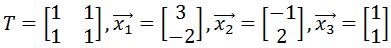
        Step 1: Understanding the Given Information

        We are provided with a transformation matrix TT and three vertices. These vertices form a shape, which in this case is a triangle. The goal is to apply the transformation matrix to these vertices to find the new, transformed vertices.

        Step 2: Representing the Vertices as a Matrix

        To proceed, we need to combine the three vertices into a single matrix. Let's denote this matrix as AA. The vertices given are (3, -2), (-1, 2), and (1, 1). We arrange these vertices into matrix AA as follows:

        \[ A = \begin{pmatrix} 3 & -1 & 1 <br/><br/> -2 & 2 & 1 \end{pmatrix} \]

        Step 3: Multiplying the Transformation Matrix by the Vertices Matrix

        Next, we need to multiply the transformation matrix TT by the vertices matrix AA. The transformation matrix TT is given as:

        \[ T = \begin{pmatrix} 1 & 1 <br/><br/> 1 & 1 \end{pmatrix} \]

        We perform the matrix multiplication T×AT \times A to find the transformed vertices.

        Step 4: Performing the Matrix Multiplication

        To find the first entry of the resulting matrix, we take the dot product of the first row of TT and the first column of AA:

        \[ (1 \times 3) + (1 \times -2) = 3 - 2 = 1 \]

        For the second entry, we take the dot product of the first row of TT and the second column of AA:

        \[ (1 \times -1) + (1 \times 2) = -1 + 2 = 1 \]

        For the third entry, we take the dot product of the first row of TT and the third column of AA:

        \[ (1 \times 1) + (1 \times 1) = 1 + 1 = 2 \]

        We repeat the same process for the second row of TT with each column of AA:

        \[ (1 \times 3) + (1 \times -2) = 3 - 2 = 1 \]

        \[ (1 \times -1) + (1 \times 2) = -1 + 2 = 1 \]

        \[ (1 \times 1) + (1 \times 1) = 1 + 1 = 2 \]

        Step 5: Interpreting the Result

        After performing the matrix multiplication, we obtain the transformed vertices matrix:

        \[ T \times A = \begin{pmatrix} 1 & 1 & 2 <br/><br/> 1 & 1 & 2 \end{pmatrix} \]

        This matrix represents the new coordinates of the vertices after the transformation. The transformed vertices are (1, 1), (1, 1), and (2, 2).

        Step 6: Conclusion

        We have successfully applied the transformation matrix to the given vertices and found the new transformed vertices. The original vertices (3, -2), (-1, 2), and (1, 1) have been transformed to (1, 1), (1, 1), and (2, 2) respectively.

        FAQs

        1. What is a transformation matrix?

          A transformation matrix is a mathematical tool used to perform geometric transformations on shapes or objects in computer graphics. It's typically a 2x2 or 3x3 matrix for 2D transformations, or a 4x4 matrix for 3D transformations. These matrices can represent various operations such as scaling, rotation, translation, or a combination of these.

        2. How do you apply a transformation matrix to a shape?

          To apply a transformation matrix to a shape, you multiply the matrix by each vertex of the shape. In practice, this is done by creating a matrix of all vertices (where each column represents a vertex) and then multiplying the transformation matrix by this vertex matrix. The resulting matrix contains the transformed coordinates of all vertices.

        3. What are the common types of transformations used in computer graphics?

          The most common transformations in computer graphics are:

          • Translation: Moving an object to a new position
          • Rotation: Changing the orientation of an object
          • Scaling: Changing the size of an object
          • Reflection: Flipping an object across an axis
          • Shear: Slanting an object
          These can be combined to create more complex transformations.

        4. Why is the order of matrix operations important in transformations?

          The order of matrix operations is crucial because matrix multiplication is not commutative. This means that applying transformations in different orders can lead to different results. For example, rotating an object and then translating it will produce a different outcome than translating it first and then rotating it. Understanding this principle is essential for achieving desired transformations in computer graphics and animation.

        5. How are matrix transformations used in real-world applications?

          Matrix transformations have numerous real-world applications:

          • In video games and 3D animation for character and object movement
          • In computer-aided design (CAD) for modeling and manipulating 3D objects
          • In robotics for controlling the movement of robotic arms
          • In image processing for operations like resizing, rotating, or skewing images
          • In augmented reality for placing virtual objects in real-world environments
          These applications demonstrate the versatility and importance of matrix transformations in modern technology and design.

        Prerequisite Topics

        Understanding the foundations of matrix operations and transformations is crucial when delving into the topic of transforming shapes with matrices. This advanced concept builds upon several key prerequisite topics that provide the necessary groundwork for comprehending how matrices can be used to manipulate geometric shapes in various ways.

        One of the fundamental prerequisites is mastering the properties of matrix multiplication. This topic is essential because matrix multiplication forms the backbone of how transformations are applied to shapes. By understanding the rules and characteristics of matrix multiplication, students can grasp how different matrices can be combined to create complex transformations.

        Another critical prerequisite is finding the transformation matrix. This skill is directly applicable to transforming shapes, as it involves determining the specific matrix that will produce a desired transformation. Whether it's a rotation, scaling, or reflection, knowing how to construct the appropriate transformation matrix is key to manipulating shapes effectively.

        Additionally, familiarity with combining transformations of functions is highly relevant. While this concept may initially focus on functions, the principles of combining multiple transformations directly translate to working with matrices and shapes. Understanding how different transformations interact and can be sequenced is crucial for creating complex shape manipulations.

        These prerequisite topics form a solid foundation for exploring the world of transforming shapes with matrices. Matrix multiplication allows students to understand how transformations are mathematically represented and applied. The ability to find transformation matrices enables the creation of specific desired changes to shapes. Lastly, knowledge of combining transformations empowers students to create intricate and multi-step shape manipulations.

        By mastering these prerequisites, students will be well-equipped to tackle the challenges of transforming shapes with matrices. They will understand the underlying mathematical principles, be able to construct and apply appropriate transformation matrices, and have the skills to combine multiple transformations for more complex shape manipulations. This comprehensive understanding not only facilitates learning the main topic but also provides valuable problem-solving skills applicable in various fields, from computer graphics to engineering and beyond.

        Let vertices of a square be vertices of a square and TT be a transformation matrix.
        Then we can transform the square by combining the vertices into a matrix (denoted by AA), and multiply it by the transformation matrix TT. In other words,
        vertices of a square in a matrix

        And TATA is the transformed square.
        Of course, this idea can also apply to other shapes other than squares.