Overview
Watch
Read
Next Steps
Watch
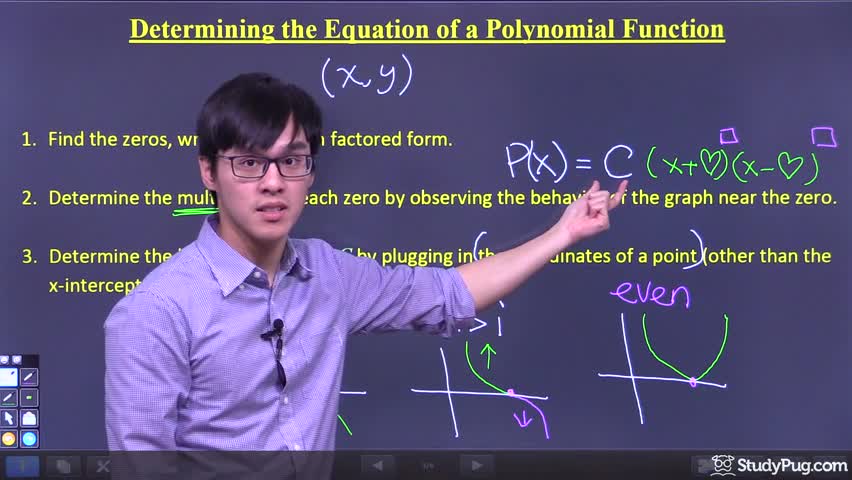
Three steps to find a polynomial equation from its graph
📝 My Notes
Auto-saves the current timestamp
Three steps to find a polynomial equation from its graph
5:05
About this lesson
Steps to Finding the Equation of a Polynomial Function
Key Moments
No key moments available.
Video 1 of 4
Three steps to find a polynomial equation from its graph
5 min
• Selected
Finding a polynomial equation from its graph using zeros and a point
6 min
Finding a polynomial equation from a graph using zeros and a point
3 min
Finding a polynomial equation from a graph with mixed multiplicities
8 min