Finding a logarithmic function given its graph

0/1
?
Intros
Lessons
  1. Introduction to finding logarithmic function given its graph

    i. What is a logarithmic function?

    ii. How can we determine the equation of a logarithmic graph?

0/8
?
Examples
Lessons
  1. Determining the Equation of an Exponential Function Given Its Graph

    Determine an exponential function in the form y=logbxy = \log_{b} x with the given graph.

    Determining the Equation of an Exponential Function Given Its Graph
    1. Determining the Equation of a Transformed Logarithmic function given its Graph

      Determine a logarithmic function in the form y=log2(x+b)+cy = \log_{2} (x + b) + c for each of the given graphs.

      1. Determining the Equation of a Transformed Logarithmic function given its Graph
      2. Determining the Equation of a Transformed Logarithmic function given its Graph
    2. Determining the Equation of a Transformed Logarithmic function given its Graph - Continued

      Determine a logarithmic function in the form y=Alog2(Bx)y = A \log_{2} (Bx) for each of the given graphs.

      1. Determining the Equation of a Transformed Logarithmic function given its Graph - Continued
      2. Determining the Equation of a Transformed Logarithmic function given its Graph - Continued
      3. Determining the Equation of a Transformed Logarithmic function given its Graph - Continued
      4. Determining the Equation of a Transformed Logarithmic function given its Graph - Continued
    3. Determining the Equation of a Logarithmic Graph With Multiple Transformations

      Determine a logarithmic function in the form y=Alog(Bx+1)+Cy = A \log (Bx+1)+C for each of the given graphs.

      Determining the Equation of a Logarithmic Graph With Multiple Transformations
      Topic Notes
      ?

      Introduction

      Finding a logarithmic function from its graph is a crucial skill in mathematics. This topic explores the process of identifying key features and using them to construct the equation of a logarithmic function. The introduction video serves as an essential starting point, providing a visual and conceptual foundation for understanding logarithmic graphs characteristics. By watching this video, students can grasp the fundamental characteristics of logarithmic functions, such as their shape, asymptotes, and intercepts. Logarithmic graphs characteristics play a significant role in various fields, including science, engineering, and economics. They are particularly useful for modeling phenomena that exhibit exponential decay modeling. Mastering the ability to interpret and derive logarithmic functions from graphs enhances problem-solving skills and deepens mathematical understanding. This knowledge is invaluable for advanced mathematical concepts and real-world applications, making it a cornerstone of mathematical education.

      Understanding the General Logarithmic Function

      Let's dive into the fascinating world of general logarithmic functions! The general equation of a logarithmic function is y = log_b(x), where 'b' is the base of the logarithm. This equation might look intimidating at first, but don't worry we'll break it down together.

      In this equation, 'x' is our input value, and 'y' is the output. The base 'b' is a positive number not equal to 1. Common bases include 10 (common logarithm), e (natural logarithm), and 2 (binary logarithm). Each base gives the logarithm its unique properties, but they all share some fundamental characteristics.

      Now, let's visualize the logarithmic function on a graph. The shape of a logarithmic graph is quite distinctive and has some key features that set it apart from other functions. Picture a curve that starts near the y-axis and gradually rises as it moves to the right. This curve never quite touches the y-axis, which leads us to one of its most important characteristics: the vertical asymptote.

      The vertical asymptote of a logarithmic function always occurs at x = 0. This means the curve gets infinitely close to the y-axis but never actually reaches or crosses it. It's like trying to reach the end of a rainbow no matter how far you walk, you can never quite get there!

      Another crucial point on our logarithmic graph is (1, 0). This point is special because it's where the curve intersects the x-axis. It tells us that log_b(1) always equals 0, regardless of the base. This makes sense when we think about exponents: any number raised to the power of 0 equals 1.

      As we move right on the graph, the curve continues to rise, but at a decreasing rate. This is why logarithmic functions are often used to model scenarios where growth slows over time, like the intensity of earthquakes or the acidity of solutions.

      One more interesting feature of logarithmic graphs is their symmetry with exponential functions. If you were to draw the line y = x and then reflect a logarithmic curve over this line, you'd get its corresponding exponential function. It's like they're mirror images of each other!

      Understanding the general logarithmic function and its graph is crucial in many fields, from mathematics and physics to economics and social sciences. It helps us model and analyze various phenomena that exhibit this particular growth pattern.

      Remember, while the equation y = log_b(x) might seem abstract, its graph tells a story of gradual, slowing growth. From its vertical asymptote at x = 0 to its steady climb through the point (1, 0) and beyond, each part of the logarithmic curve represents a unique mathematical relationship.

      As you continue your journey in mathematics, you'll find that logarithmic functions are powerful tools for solving complex problems and understanding intricate relationships in our world. Keep exploring, and don't hesitate to graph these functions yourself practice makes perfect!

      Identifying Transformations in Logarithmic Graphs

      Understanding transformations in logarithmic graphs is crucial for analyzing and interpreting these important mathematical functions. In this section, we'll explore how to recognize horizontal and vertical shifts in logarithmic graphs, and how these transformations affect key features of the graph, such as the vertical asymptote and y-intercept.

      Logarithmic graphs are characterized by their distinctive shape, with a vertical asymptote on one side and a gradually increasing or decreasing curve on the other. The basic form of a logarithmic function is y = logb(x), where b is the base of the logarithm. When we apply transformations to this basic form, we can shift the graph horizontally or vertically, changing its position on the coordinate plane.

      Let's start by examining horizontal shifts in logarithmic graphs. A horizontal shift occurs when we add or subtract a constant inside the logarithm. The general form for a horizontally shifted logarithmic function is y = logb(x - h), where h represents the horizontal shift. If h is positive, the graph shifts h units to the right, and if h is negative, the graph shifts |h| units to the left.

      To recognize a horizontal shift in a logarithmic graph, look for changes in the position of the vertical asymptote. The vertical asymptote of a logarithmic function occurs where the input value would make the logarithm undefined typically when the input is zero or negative. In the case of a horizontal shift, the vertical asymptote will move along the x-axis. For a right shift, the asymptote moves right, and for a left shift, it moves left.

      For example, consider the function y = log2(x - 3). This function is shifted 3 units to the right compared to the basic function y = log2(x). The vertical asymptote, which was originally at x = 0, is now at x = 3. Similarly, for y = log2(x + 2), the graph is shifted 2 units to the left, and the vertical asymptote is at x = -2.

      Vertical shifts, on the other hand, occur when we add or subtract a constant outside the logarithm. The general form for a vertically shifted logarithmic function is y = logb(x) + k, where k represents the vertical shift. If k is positive, the graph shifts k units up, and if k is negative, the graph shifts |k| units down.

      To recognize a vertical shift in a logarithmic graph, observe changes in the y-intercept. The y-intercept of a logarithmic function is the point where the graph crosses the y-axis, typically when x = 1 (since logb(1) = 0 for any base b). In a vertical shift, the entire graph moves up or down, including the y-intercept.

      For instance, the function y = log2(x) + 3 is shifted 3 units up compared to y = log2(x). The y-intercept, which was originally at (1, 0), is now at (1, 3). Conversely, y = log2(x) - 2 is shifted 2 units down, with the y-intercept at (1, -2).

      It's important to note that vertical shifts do not affect the position of the vertical asymptote. The asymptote remains at the same x-value, regardless of the vertical transformation. This is because the vertical asymptote is determined by the input values that make the logarithm undefined, which are not changed by adding or subtracting a constant outside the logarithm.

      Let's look at a more complex example that combines both horizontal and vertical shifts: y = log3(x + 2) - 1. This function undergoes two transformations: a horizontal shift of 2 units to the left (x + 2 inside the logarithm) and a vertical shift of 1 unit down. This is an example of combined horizontal and vertical shifts in logarithmic functions.

      Steps to Find the Logarithmic Function from a Graph

      Determining the equation of a logarithmic function from its graph is a crucial skill in mathematics. This process involves carefully analyzing the graph's features and translating them into a mathematical formula. Let's outline a step-by-step approach to find the log graph formula, which will help you master this important concept.

      Step 1: Identify the Parent Function

      Begin by recognizing the basic shape of the logarithmic function. The parent function for a logarithmic graph is y = log(x) or y = ln(x) for natural logarithms. This will serve as your starting point.

      Step 2: Determine the Base

      Look at the graph to identify the base of the logarithm. If the curve passes through the point (1, 0), it's likely a natural logarithm (base e). If it passes through (10, 1), it's probably a common logarithm (base 10). For other bases, you'll need to analyze additional points.

      Step 3: Locate the Vertical Asymptote

      Find the vertical line that the graph approaches but never crosses. This line represents the vertical asymptote and will help you determine any horizontal shifts in the function. The equation of this asymptote is x = a, where 'a' is the x-intercept of the asymptote.

      Step 4: Identify Horizontal Shifts

      If the vertical asymptote is not at x = 0, there's a horizontal shift. The amount of shift is equal to 'a' from Step 3. Your equation will include (x - a) inside the logarithm.

      Step 5: Determine Vertical Shifts

      Check if the graph intersects the y-axis at a point other than (0, 0). If it does, there's a vertical shift. Add or subtract this value (let's call it 'k') to your equation.

      Step 6: Identify Reflections

      If the graph opens to the left instead of the right, there's a reflection over the y-axis. This is represented by a negative sign before the logarithm.

      Step 7: Look for Vertical Stretches or Compressions

      Compare the steepness of your graph to the parent function. A steeper curve indicates a vertical stretch, while a flatter curve suggests a compression. This is represented by a coefficient 'c' in front of the logarithm.

      Step 8: Combine All Transformations

      Put all the identified transformations together to form your equation: y = c * log_b(x - a) + k, where 'b' is the base, 'c' is the vertical stretch/compression factor, 'a' is the horizontal shift, and 'k' is the vertical shift.

      Example: Analyzing a Logarithmic Graph

      Let's walk through an example to illustrate this process. Suppose we have a logarithmic graph with the following characteristics:

      • The curve passes through (1, 0), indicating it's a natural logarithm (base e).
      • The vertical asymptote is at x = 2, suggesting a horizontal shift of 2 units right.
      • The graph intersects the y-axis at (0, 1), indicating a vertical shift of 1 unit up.
      • The curve is twice as steep as the parent function, suggesting a vertical stretch by a factor of 2.

      Following our steps:

      1. Parent function: y = ln(x)
      2. Base: e (natural logarithm)
      3. Vertical asymptote: x = 2
      4. Horizontal shift: 2 units right
      5. Vertical shift: 1 unit up
      6. Vertical stretch: factor of 2
      7. Reflection: none

      Practice Problems and Solutions

      Let's dive into some practice problems to help you master the skill of finding logarithmic functions from graphs. Before we begin, remember that a logarithmic function has the general form f(x) = a logb(x - h) + k, where a is the vertical stretch factor, b is the base, h is the horizontal shift, and k is the vertical shift. Try to solve these problems on your own before checking the solutions!

      Problem 1:

      Given a graph that passes through the points (1, 0), (2, 1), and (4, 2), find the logarithmic function.

      Problem 2:

      A logarithmic curve passes through (1, 2) and (e, 3). The vertical asymptote is at x = -1. Determine the function.

      Problem 3:

      Find the logarithmic function for a graph with a vertical asymptote at x = 2, passing through the point (6, 1), and with a vertical stretch factor of 2.

      Solutions:

      Solution 1:

      Step 1: Identify the base. Since f(2) = 1, we can deduce that the base is 2.
      Step 2: The point (1, 0) suggests there's no vertical shift (k = 0).
      Step 3: There's no horizontal shift (h = 0) as the curve passes through (1, 0).
      Step 4: Use f(4) = 2 to find a: 2 = a log2(4), so a = 1.
      Therefore, the function is f(x) = log2(x).

      Solution 2:

      Step 1: The vertical asymptote at x = -1 indicates h = 1 (shift right).
      Step 2: Use the point (1, 2): 2 = a ln(1 - 1) + k, so k = 2.
      Step 3: Use (e, 3): 3 = a ln(e - 1) + 2, so a = 1.
      The function is f(x) = ln(x - 1) + 2.

      Solution 3:

      Step 1: Vertical asymptote at x = 2 means h = -2 (shift left).
      Step 2: Given vertical stretch factor a = 2.
      Step 3: Use (6, 1): 1 = 2 logb(6 - (-2)) + k, so 1 = 2 logb(8) + k.
      Step 4: Try b = 2: 1 = 2 * 3 + k, so k = -5.
      The function is f(x) = 2 log2(x + 2) - 5.

      Practice these problems using a log grapher to visualize the curves and check your answers. Remember, finding the logarithmic curve equation requires careful analysis of key points, asymptotes, and transformations. As you work through more problems, you'll develop a better intuition for identifying these crucial elements from graphs.

      To further improve your skills, try creating your own practice problems. Start with a logarithmic function, graph it using a log grapher, and then challenge yourself or a study partner to derive the function from the graph. This reverse-engineering process can significantly enhance your understanding of logarithmic functions and their graphical representations.

      Keep in mind that real-world applications often involve logarithmic relationships. For instance, the Richter scale for measuring earthquake intensity and the decibel scale for sound intensity both use logarithmic scales. By mastering these concepts, you're not just solving abstract math problems

      Common Mistakes and How to Avoid Them

      When it comes to finding logarithmic functions from graphs, students often encounter several common pitfalls. Let's explore these mistakes and learn how to avoid them, so you can master this important mathematical skill. One frequent error is misinterpreting the y-intercept of the logarithmic function. Remember, the y-intercept always occurs at x = 1, not x = 0 as in many other functions. This is because the domain of a logarithmic function starts at x > 0. To avoid this, always double-check that you're reading the y-value at x = 1 for the y-intercept.

      Another common mistake is confusing the base of the logarithm. The base determines the shape and behavior of the function, so it's crucial to identify it correctly. Look for the point where the function crosses y = 0; the x-coordinate at this point is the base of the logarithm. If you're having trouble with this, try plotting a few known logarithmic functions to familiarize yourself with how different bases affect the graph's appearance.

      Students often struggle with identifying vertical asymptote of logarithmic functions. Remember, the vertical asymptote always occurs at x = 0 for standard logarithmic functions. If you see the graph approaching but never quite reaching a vertical line, that's your asymptote! To avoid mistakes, always start by locating this crucial feature of the graph.

      Misreading the direction of the function is another common error. Logarithmic functions can either increase from left to right (for bases greater than 1) or decrease (for bases between 0 and 1). Pay close attention to the overall trend of the graph to determine this. If you're unsure, try plotting a few points to confirm the direction.

      Lastly, students sometimes forget that logarithmic functions are the inverse of exponential functions. This relationship can be incredibly helpful when analyzing graphs. If you're having trouble interpreting a logarithmic graph, try thinking about how its exponential counterpart would behave. This mental flip can often provide valuable insights and help you avoid mistakes.

      Remember, making mistakes is a natural part of the learning process. Don't get discouraged if you find yourself stumbling on these concepts. With practice and attention to detail, you'll soon become proficient at analyzing logarithmic graphs. Keep these tips in mind, take your time when analyzing graphs, and don't hesitate to ask for help when needed. You've got this!

      Real-world Applications of Logarithmic Functions

      Logarithmic functions play a crucial role in various fields, offering practical applications that extend far beyond mathematical theory. In science, finance, and technology, these functions provide invaluable tools for analyzing and interpreting complex phenomena. Understanding logarithmic graphs can be immensely useful in real-life scenarios, allowing us to make sense of data that spans multiple orders of magnitude.

      In the realm of science, logarithmic functions are indispensable. For instance, in seismology, the Richter scale uses logarithms to measure earthquake intensity. This logarithmic scale allows scientists to compare earthquakes of vastly different magnitudes on a single, comprehensible scale. Similarly, in chemistry, pH levels are measured using a logarithmic scale, enabling precise comparisons of acidity and alkalinity across a wide range.

      The field of finance heavily relies on logarithmic functions, particularly in analyzing long-term trends and compound interest. Logarithmic charts are often used to visualize stock prices over extended periods, as they can effectively display percentage changes rather than absolute values. This makes it easier to compare relative performance across different time frames. Moreover, compound interest calculations, fundamental to investment planning and loan amortization, are based on exponential growth, which is closely related to logarithmic functions.

      In technology, logarithmic functions find applications in various areas. Audio engineers use decibels, a logarithmic unit, to measure sound intensity. This logarithmic scale aligns more closely with human perception of loudness than a linear scale would. In computer science, algorithms often employ logarithmic time complexity, such as in binary search trees, which are crucial for efficient data retrieval and sorting operations.

      Understanding logarithmic graphs is particularly useful when dealing with data that spans several orders of magnitude. For example, in astronomy, the brightness of stars is measured on a logarithmic scale, allowing astronomers to compare the luminosity of extremely bright and dim stars on the same chart. In biology, population growth models often follow logarithmic patterns, helping ecologists predict and analyze species dynamics over time.

      The ability to interpret logarithmic scales is also valuable in everyday life. For instance, understanding decibel levels can help in assessing noise pollution or choosing appropriate hearing protection. In the current global health context, logarithmic graphs have been widely used to track the spread of infectious diseases, providing a clear visualization of exponential growth rates.

      By grasping the principles of logarithmic functions and their graphical representations, individuals can better interpret complex data, make informed decisions, and gain deeper insights into various natural and man-made phenomena. Whether in scientific research, financial analysis, or technological innovation, logarithmic functions continue to be indispensable tools for understanding and navigating our complex world.

      Conclusion

      In this article, we've explored the fascinating world of logarithmic functions and their graphical representations. We've learned how to identify these functions from their distinctive curved shapes and asymptotic behavior. The introduction video provided a crucial foundation for understanding these concepts, making it an essential starting point for anyone new to the topic. As you continue your journey with logarithmic functions, practice is key. Challenge yourself to identify these functions from various graphs, paying close attention to their unique characteristics. Remember, the more you engage with these concepts, the more intuitive they'll become. We encourage you to explore further resources, solve practice problems, and discuss your findings with peers or instructors. By mastering logarithmic functions and their graphs, you'll unlock a powerful tool for analyzing exponential growth and decay in various real-world applications. Keep exploring, and don't hesitate to revisit this article and the introductory video as needed to reinforce your understanding.

      Example:

      Determining the Equation of a Transformed Logarithmic function given its Graph

      Determine a logarithmic function in the form y=log2(x+b)+cy = \log_{2}(x + b) + c for each of the given graphs.

      Determining the Equation of a Transformed Logarithmic function given its Graph

      Step 1: Understanding the Form of the Logarithmic Function

      We start by understanding the form of the logarithmic function we need to determine. The function is given in the form y=log2(x+b)+cy = \log_{2}(x + b) + c. Here, bb represents the horizontal shift, and cc represents the vertical shift. Our goal is to find the values of bb and cc that transform the reference graph y=log2(x)y = \log_{2}(x) to match the given graph.

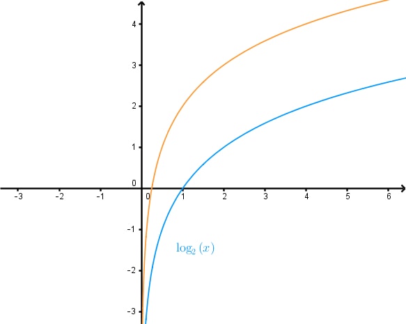
      Step 2: Analyzing the Reference Graph

      We use the reference graph of y=log2(x)y = \log_{2}(x) to understand the transformations. The reference graph passes through the point (1, 0) and has a vertical asymptote at x=0x = 0. This information helps us identify any shifts in the given graph.

      Step 3: Identifying the Vertical Asymptote

      Next, we examine the vertical asymptote of the given graph. If the vertical asymptote remains at x=0x = 0, it indicates that there is no horizontal shift. In this case, the value of bb would be 0. If the vertical asymptote has shifted, we would need to determine the value of bb accordingly.

      Step 4: Determining the Horizontal Shift (b)

      In the given graph, the vertical asymptote is still at x=0x = 0. This means there is no horizontal translation, and thus, b=0b = 0. We can now update our function to y=log2(x)+cy = \log_{2}(x) + c.

      Step 5: Identifying the Vertical Shift (c)

      To determine the vertical shift, we look at how the points on the reference graph have moved vertically. We observe that each point on the reference graph has been translated vertically by a certain number of units. By counting the units of vertical translation, we can determine the value of cc.

      Step 6: Calculating the Vertical Shift (c)

      We notice that every point on the reference graph has been shifted vertically by 2 units upwards. This means the value of cc is 2. Therefore, our updated function becomes y=log2(x)+2y = \log_{2}(x) + 2.

      Step 7: Verifying the Transformation

      Finally, we verify our transformation by checking if the updated function y=log2(x)+2y = \log_{2}(x) + 2 matches the given graph. We ensure that the vertical asymptote remains at x=0x = 0 and that all points have been shifted correctly by 2 units upwards.

      Conclusion

      By following these steps, we have determined the equation of the transformed logarithmic function given its graph. The function is in the form y=log2(x+b)+cy = \log_{2}(x + b) + c, where b=0b = 0 and c=2c = 2. This process can be applied to other graphs to find their corresponding logarithmic functions.

      FAQs

      Here are some frequently asked questions about finding logarithmic functions from graphs:

      1. What type of graph is logarithmic?

      A logarithmic graph has a distinctive curved shape that starts with a steep increase (or decrease) and gradually levels off. It has a vertical asymptote on one side and extends infinitely in the other direction, never crossing the asymptote.

      2. What is the logarithmic equation for a graph?

      The general form of a logarithmic equation is y = a logb(x - h) + k, where 'a' is the vertical stretch factor, 'b' is the base of the logarithm, 'h' is the horizontal shift, and 'k' is the vertical shift.

      3. How do you tell if a graph is exponential or logarithmic?

      Logarithmic graphs have a vertical asymptote and level off as x increases, while exponential graphs have a horizontal asymptote and grow increasingly steep as x increases. Logarithmic graphs are essentially the reflection of exponential graphs over the line y = x.

      4. What are the 4 steps to graph a log function?

      1) Identify the vertical asymptote (x = h). 2) Plot the y-intercept (0, k). 3) Use the change of base formula to plot additional points. 4) Connect the points with a smooth curve that approaches but never touches the vertical asymptote.

      5. How do you write the equation for a logarithmic function from a graph?

      To write the equation: 1) Identify the vertical asymptote to find 'h'. 2) Locate the y-intercept to determine 'k'. 3) Use two points to calculate 'a' and 'b'. 4) Combine these elements into the general form y = a logb(x - h) + k.

      Prerequisite Topics

      Understanding the prerequisite topics is crucial when learning how to find a logarithmic function given its graph. These foundational concepts provide the necessary background to interpret and analyze logarithmic graphs effectively.

      One of the key prerequisites is understanding the characteristics of polynomial graphs. While logarithmic functions are not polynomials, many of the graphing principles apply, such as identifying key points and understanding how the function behaves. This knowledge helps in recognizing the unique shape and properties of logarithmic graphs.

      The concept of continuous growth and decay is particularly relevant to logarithmic functions. Logarithmic graphs often represent scenarios of continuous growth or decay, making this prerequisite essential for interpreting real-world applications of these functions.

      Understanding vertical asymptotes is crucial when working with logarithmic graphs. Logarithmic functions typically have a vertical asymptote, and recognizing this feature is key to accurately sketching and analyzing these graphs.

      While more advanced, knowledge of the derivative of logarithmic functions can provide insights into the rate of change and behavior of these functions, which can be helpful in understanding their graphs.

      The concept of reflection across the y-axis is important when dealing with different forms of logarithmic functions, particularly when comparing graphs of logarithms with different bases.

      Understanding horizontal and vertical distances on a graph is fundamental to interpreting logarithmic scales and transformations of logarithmic functions.

      Familiarity with logarithmic scales, such as the dB scale, provides practical context for logarithmic functions and enhances understanding of their real-world applications.

      By mastering these prerequisite topics, students will be better equipped to analyze and interpret logarithmic graphs, making the process of finding a logarithmic function from its graph more intuitive and manageable. Each of these concepts contributes to a comprehensive understanding of logarithmic behavior, enabling students to approach more complex problems with confidence and clarity.