Overview
Watch
Read
Next Steps
Watch
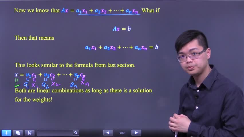
Intro to the matrix equation Ax=b and matrix-vector multiplication
📝 My Notes
Auto-saves the current timestamp
Intro to the matrix equation Ax=b and matrix-vector multiplication
8:03
About this lesson
• Product of \(A\) and \(x\)
• Multiplying a matrix and a vector
• Relation to Linear combination
Key Moments
No key moments available.
Video 1 of 12
Intro to the matrix equation Ax=b and matrix-vector multiplication
8 min
• Selected
Writing a system of equations in matrix equation form Ax=b
4 min
Converting a matrix equation Ax=b into an augmented matrix to solve
3 min
Properties of the matrix-vector product Ax
6 min
Multiplying a 3x2 matrix by a 2-entry vector using Ax=b
4 min
Computing Ax=b with a 3-column matrix and 3-entry vector
5 min
Why Ax=b fails when column count doesn't match vector entries
3 min
Converting a system of equations to vector and matrix equation form
8 min
Solving Ax=b by forming an augmented matrix and row reducing
11 min
Solving a 3x3 matrix equation using row reduction
18 min
Showing Ax=b has solutions for some b and no solution for others
9 min
Proving a matrix-vector equation using properties of Ax
8 min