Interval of validity

Get the most by viewing this topic in your current grade. Pick your course now.

?
Intros
Lessons
  1. What is an interval of validity?
?
Examples
Lessons
  1. Determining Intervals of Validity
    For each of the following differential equations, the corresponding slope field is provided.
    Sketch the solution for each differential equation with the specific initial conditions given. What is the interval of validity?
    1. dydx=1(x+1),y(0)=2 \frac{dy}{dx}=\frac{1}{(x+1)}, y(0)=2
      Determining the interval of validity with slope fields
    2. dydx=e2x2+2y,y(4)=4 \frac{dy}{dx}=e^{-2x^2}+2y, y(-4)=4
      Slope fields and interval of validity
  2. In the section to do with Bernoulli Equations the solution to the differential equation:

    dydx+1xy=y3\frac{dy}{dx}+\frac{1}{x} y=y^3

    with initial condition y(12)=1y(\frac{1}{2})=1 was found to be:

    y=12xy=\frac{1}{\sqrt{2x}}

    Plot out this solution and explicitly give its interval of validity.
    1. Solve the following differential equation:

      dydx=2xey\frac{dy}{dx}=-2xe^{-y}

      With initial conditions y(1)=0y(1)=0.

      What is the interval of validity for the solution?
      1. Solve the following differential equation:

        dydx=4xy2\frac{dy}{dx}=4xy^2
        1. What is the interval of validity with initial conditions y(0)=12y(0)=\frac{1}{2}?
        2. What is the interval of validity with initial conditions y(12)=2y(\frac{1}{2})=-2?
      Topic Notes
      ?

      Introduction to Interval of Validity

      The interval of validity is a fundamental concept in differential equations, crucial for understanding the range where a solution remains valid. Our introduction video serves as an essential starting point, providing a clear and concise explanation of this important topic. In differential equations, solutions are not always applicable across all values; the interval of validity defines the specific range where a solution holds true. This concept is vital for accurately interpreting and applying differential equation solutions in various fields, including physics, engineering, and economics. By grasping the interval of validity, students and professionals can avoid misapplying solutions outside their intended range, ensuring more accurate and reliable results in their calculations and models. The introduction video breaks down this complex topic into easily digestible segments, making it an invaluable resource for both beginners and those looking to refresh their knowledge in this critical area of mathematics.

      Understanding Interval of Validity

      The interval of validity is a crucial concept in the study of differential equations, playing a significant role in determining the range where a solution is meaningful and continuous. In the context of differential equations, this interval represents the domain where the solution function is well-defined and behaves as expected. Understanding the interval of validity is essential for accurately solving and interpreting differential equations in various scientific and engineering applications.

      When we solve a differential equation, we're essentially finding a function that satisfies the given equation and initial conditions. However, this solution may not be valid for all possible input values. The interval of validity defines the specific range of inputs where the solution remains continuous and adheres to the differential equation's constraints. Outside this interval, the solution may become undefined, discontinuous, or violate the equation's conditions.

      To illustrate this concept, let's consider an example from a typical differential equations problem. Imagine we have the differential equation dy/dx = y^2, with the initial condition y(0) = 1. Using separation of variables and integration, we can derive the general solution y = -1 / (x - C), where C is a constant determined by the initial condition. Applying the initial condition y(0) = 1, we find that C = 1, giving us the particular solution y = -1 / (x - 1).

      Now, let's examine the interval of validity for this solution. We can see that the function y = -1 / (x - 1) has a vertical asymptote at x = 1. This means that as x approaches 1, the value of y approaches infinity, creating a discontinuity. Therefore, the interval of validity for this solution is (-, 1), excluding the point x = 1 where the function is undefined.

      The concept of interval of validity is closely related to initial conditions and slope fields. Initial conditions provide a starting point for the solution, often determining the specific form of the solution function. Slope fields, which visually represent the direction and magnitude of the derivative at various points, can help us identify potential issues with continuity and validity across different regions of the solution space.

      Understanding the interval of validity is crucial for several reasons. First, it helps us recognize the limitations of our solutions and avoid applying them in contexts where they're not valid. Second, it allows us to anticipate and handle potential singularities or discontinuities in the solution. Finally, it provides insight into the behavior of the system described by the differential equation, including any physical or mathematical constraints that might limit the solution's applicability.

      In practice, determining the interval of validity often involves analyzing the solution function for potential issues such as division by zero, undefined logarithms, or square roots of negative numbers. It's also important to consider any physical constraints or assumptions made in deriving the differential equation, as these may further restrict the valid range of the solution.

      By mastering the concept of interval of validity, students and practitioners of differential equations can ensure that their solutions are applied correctly and interpreted accurately within the appropriate domain. This understanding forms a fundamental part of the broader skill set required for solving and analyzing differential equations in various scientific and engineering disciplines.

      Graphical Representation of Interval of Validity

      Visualizing the interval of validity using graphs and slope fields is a powerful technique in understanding differential equations. Slope fields, also known as direction fields, provide a graphical representation of the solutions to a differential equation without actually solving it. This method is particularly useful in determining the behavior of solutions and their intervals of validity.

      To create a slope field, we start by considering a differential equation in the form dy/dx = f(x,y). The process involves plotting short line segments at various points in the xy-plane, where each segment represents the slope of the solution curve at that point. These segments are drawn according to the slope given by the differential equation at each point.

      For example, let's consider the differential equation dy/dx = x - y. To draw its slope field, we would calculate the slope at various points (x,y) and draw short line segments with those slopes. At the point (1,1), the slope would be 1 - 1 = 0, so we'd draw a horizontal line segment. At (2,1), the slope would be 2 - 1 = 1, so we'd draw a line segment at a 45-degree angle.

      Once the slope field is drawn, we can visualize the general behavior of solution curves without solving the equation explicitly. Solution curves are paths that follow the direction of the slope field at every point. By tracing a curve that is always tangent to the line segments in the slope field, we can sketch approximate solution curves.

      The interval of validity becomes apparent when we examine these solution curves in the context of the slope field. It represents the range over which a particular solution exists and remains well-defined. Graphically, this interval corresponds to the portion of the x-axis where the solution curve can be continuously drawn without encountering any singularities or undefined behavior.

      Initial conditions play a crucial role in determining the specific solution curve and, consequently, its interval of validity. When given an initial condition (x, y), we start tracing the solution curve from that point, following the slope field. The interval of validity for this particular solution extends from the initial x-value until we reach a point where the solution can no longer be continued or becomes undefined.

      For instance, if we have the differential equation dy/dx = 1 / (1 - x²) and an initial condition of (0,0), we would start tracing the solution curve from the origin. As we follow the slope field, we'd notice that the solution approaches infinity as x approaches 1 or -1. Therefore, the interval of validity for this solution would be (-1, 1), as the solution is well-defined within this open interval but becomes undefined at x = ±1.

      It's important to note that different initial conditions can lead to different intervals of validity for the same differential equation. Some solutions may have a finite interval of validity, while others might be valid for all real numbers. The slope field helps us visualize these differences by showing how solution curves behave across the entire xy-plane.

      In practice, software tools are often used to generate accurate slope fields and plot solution curves. These tools allow for interactive exploration of different initial conditions and their effects on the interval of validity. However, even rough sketches of slope fields can provide valuable insights into the behavior of solutions and their validity intervals.

      By combining the graphical representation of slope fields with analytical techniques, we can gain a comprehensive understanding of differential equations and their solutions. This visual approach not only aids in determining intervals of validity but also helps in developing intuition about the behavior of solutions in various regions of the xy-plane.

      Determining Interval of Validity

      Determining the interval of validity for a differential equation and its initial condition is a crucial step in understanding the solution's behavior. This step-by-step guide will help you navigate this process, ensuring you can accurately identify where the solution is valid and meaningful.

      Step 1: Understand the Concept

      The interval of validity refers to the range of values for the independent variable where the solution to a differential equation is defined and satisfies both the equation and the initial condition. It's essential to determine this interval to ensure we're working with a valid solution.

      Step 2: Solve the Differential Equation

      Begin by solving the given differential equation. This may involve integration, separation of variables, or other solving techniques depending on the equation's form.

      Step 3: Apply the Initial Condition

      Use the provided initial condition to determine any constants of integration in your general solution. This step transforms your general solution into a particular solution that satisfies both the differential equation and the initial condition.

      Step 4: Examine the Solution

      Carefully inspect your solution for potential issues that might limit its validity:

      • Discontinuities: Points where the function is not continuous
      • Breaks: Sudden jumps or gaps in the function
      • Holes: Points where the function is undefined

      Step 5: Check for Domain Restrictions

      Look for any expressions in your solution that might have restricted domains, such as square roots of negative numbers, logarithms of non-positive numbers, or divisions by zero.

      Step 6: Determine the Interval

      Based on your analysis in steps 4 and 5, determine the largest continuous interval where the solution is valid. This interval should include the initial condition and extend as far as possible without encountering any of the issues identified.

      Example: All Real Numbers

      In some cases, like the example mentioned in the video, the interval of validity might extend to all real numbers. This occurs when the solution is continuous and well-defined for every real number, without any restrictions or problematic points.

      The Impact of Initial Conditions

      It's important to note that different initial conditions can lead to different intervals of validity, even for the same differential equation. Here's why:

      • Starting Point: The initial condition determines where the solution begins, which can affect where it remains valid.
      • Singularities: Some initial conditions might lead to solutions that encounter singularities or undefined points more quickly than others.
      • Domain Restrictions: Certain initial values might result in solutions that more readily violate domain restrictions of functions involved in the solution.

      Practical Considerations

      When determining the interval of validity, consider the following:

      • Physical Context: If the differential equation models a real-world phenomenon, consider any physical constraints that might limit the validity of the solution.
      • Graphical Analysis: Plotting the solution can often provide visual insights into its behavior and potential issues.
      • Numerical Verification: For complex cases, using numerical methods to solve the differential equation at various points can help verify your analytical findings.

      Conclusion

      Determining the interval of validity is a critical step in working with differential equations. It ensures that we understand where our solution is meaningful and applicable. By carefully examining the solution for discontinuities, breaks, holes, and domain restrictions, and considering the impact of initial conditions, we can confidently establish the range over which our solution holds true. This process not only enhances our mathematical understanding but also ensures the practical applicability of our solutions in real-world scenarios.

      Existence and Uniqueness Theorem

      The Existence and Uniqueness Theorem is a fundamental concept in the study of first-order differential equations. This theorem provides crucial insights into the nature of solutions for these equations, addressing two key questions: whether a solution exists and if it is unique within a specific interval.

      To understand this theorem, we must first consider a general first-order differential equation in the form dy/dx = f(x, y), where f is a function of both x and y. The Existence and Uniqueness Theorem states that if f(x, y) and its partial derivative with respect to y, f/y, are both continuous functions in a rectangular region R containing the point (x, y), then there exists a unique solution y = φ(x) to the initial value problem:

      dy/dx = f(x, y), y(x) = y

      This solution is valid in some interval I containing x. The interval I is called the interval of validity, and it represents the range of x-values for which the solution exists and remains unique.

      The conditions of continuity for both f(x, y) and f/y are crucial for ensuring the existence and uniqueness of the solution. Continuity of f(x, y) guarantees that the differential equation is well-defined and behaves smoothly, while the continuity of f/y ensures that small changes in y lead to predictable changes in the rate of change dy/dx.

      To illustrate the importance of these conditions, let's consider an example from the video. Suppose we have the differential equation dy/dx = |y|. At first glance, this equation might seem straightforward, but it actually violates the conditions of the Existence and Uniqueness Theorem at y = 0.

      The function f(x, y) = |y| is continuous for all real y, but its partial derivative with respect to y, f/y = 1/(2|y|), is undefined when y = 0. This discontinuity in the partial derivative leads to interesting behavior near y = 0.

      If we consider the initial condition y(0) = 0, we find that there are actually multiple solutions satisfying this condition: 1. y(x) = 0 for all x 2. y(x) = (x/2)² for x 0, and y(x) = 0 for x < 0 3. y(x) = 0 for x 0, and y(x) = (x/2)² for x > 0

      This example demonstrates that when the conditions of the Existence and Uniqueness Theorem are not met, we may encounter situations where multiple solutions exist, or where solutions behave unpredictably.

      The interval of validity is closely related to the Existence and Uniqueness Theorem. It represents the largest interval containing the initial point x for which the solution remains unique. The boundaries of this interval are typically determined by: 1. Points where the solution ceases to exist (e.g., approaching infinity) 2. Points where the solution or its derivative becomes discontinuous 3. The edges of the region R where the continuity conditions are guaranteed

      Understanding the Existence and Uniqueness Theorem and its implications is crucial for analyzing differential equations and their solutions. It provides a solid foundation for numerical methods, qualitative analysis, and the development of more advanced theorems in the field of differential equations.

      In practical applications, this theorem helps engineers and scientists determine when they can rely on a unique solution to model physical phenomena accurately. It also guides the selection of appropriate numerical methods for solving differential equations in cases where analytical solutions are not available.

      By ensuring that the conditions of the theorem are met, researchers can confidently apply differential equation models to real-world problems, knowing that their solutions will be well-behaved and predictable within the interval of validity.

      Practical Applications and Examples of Interval of Validity

      The interval of validity is a crucial concept in differential equations applications, with significant implications in real-world applications. Understanding this concept is essential for students and professionals alike, particularly in fields such as physics and engineering. Let's explore additional examples and practical applications to deepen our understanding of the interval of validity.

      Example 1: Population Growth Model
      Consider the differential equation dP/dt = kP, where P represents population and k is the growth rate. Given an initial population P(0) = 1000 and k = 0.05, determine the interval of validity. In this case, the solution is valid for all positive time (0, ) since population growth is theoretically unbounded. However, in reality, factors like resource limitations would eventually restrict growth, highlighting the importance of considering real-world constraints when interpreting differential equations applications.

      Example 2: Radioactive Decay
      The equation dN/dt = -λN describes radioactive decay, where N is the number of radioactive nuclei and λ is the decay constant. For an initial amount N(0) = 1000 and λ = 0.1, the interval of validity is [0, ). This is because the decay process continues indefinitely, although the amount approaches zero asymptotically.

      Example 3: Harmonic Oscillator
      The equation d²x/dt² + ω²x = 0 represents a simple harmonic oscillator. With initial conditions x(0) = 1 and x'(0) = 0, and ω = 2π, the solution is valid for all real numbers (-, ). This illustrates how some physical systems can have solutions valid for all time, both past and future.

      Practical Application: Structural Engineering
      In structural engineering, the interval of validity is crucial when modeling the deflection of beams under load. The equation EI(dy/dx) = w(x) describes beam deflection, where E is Young's modulus, I is the moment of inertia, y is deflection, and w(x) is the load distribution. The interval of validity here is typically the length of the beam [0, L]. Understanding this interval is vital for ensuring structural integrity and safety in construction projects.

      Practical Application: Fluid Dynamics
      In fluid dynamics, the Navier-Stokes equations describe fluid motion. The interval of validity for solutions to these equations is critical in applications like weather prediction and aerodynamics. For instance, in modeling airflow around an aircraft wing, the interval of validity might be limited by factors such as air compressibility at high speeds, emphasizing the need to consider physical limitations when applying mathematical models.

      Practical Application: chemical kinetics rate law
      In chemical kinetics, the rate law dC/dt = -kC² describes a second-order reaction, where C is concentration and k is the rate constant. The interval of validity for this equation is typically [0, t_final], where t_final is when the reaction is essentially complete. Understanding this interval is crucial for accurately predicting reaction progress and optimizing industrial processes.

      Problem for Students: Heat Conduction
      Consider the heat equation T/t = α²T/x², describing heat conduction in a rod. Given initial condition T(x,0) = sin(πx/L) for 0 x L, and boundary conditions T(0,t) = T(L,t) = 0, determine the interval of validity for x and t. This problem challenges students to consider both spatial and temporal domains in defining the interval of validity.

      Understanding the interval of validity is not just a mathematical exercise; it's a fundamental skill for applying differential equations to real-world problems. It helps in recognizing the limitations of models, predicting when solutions might break down, and making informed decisions in engineering and scientific applications. By practicing with diverse examples and considering practical scenarios, students can develop a robust intuition for determining and interpreting intervals of validity in various contexts, including chemical kinetics rate law.

      Conclusion

      The interval of validity is a crucial concept in solving differential equations, defining the range where a solution remains valid and meaningful. It helps identify limitations and potential singularities in solutions. The introduction video provides a visual and intuitive understanding of this concept, making it easier for students to grasp its importance. Determining the interval of validity is essential for accurately interpreting and applying solutions to real-world problem applications. Students are encouraged to practice finding intervals of validity for various differential equations, as this skill is fundamental in advanced mathematical analysis. By mastering this concept, learners can confidently approach more complex topics in differential equations, such as boundary value problems and partial differential equations. Regular practice and exploration of diverse examples will strengthen understanding and prepare students for advanced studies in mathematics, physics, and engineering, where solving differential equations play a pivotal role in modeling complex systems and phenomena.

      Example:

      Determining Intervals of Validity
      For each of the following differential equations, the corresponding slope field is provided.
      Sketch the solution for each differential equation with the specific initial conditions given. What is the interval of validity? dydx=1(x+1),y(0)=2 \frac{dy}{dx}=\frac{1}{(x+1)}, y(0)=2
      Determining the interval of validity with slope fields

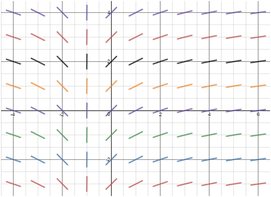
      Step 1: Understanding the Differential Equation and Initial Condition

      First, we need to understand the given differential equation and the initial condition. The differential equation provided is: \[ \frac{dy}{dx} = \frac{1}{x+1} \] with the initial condition y(0)=2 y(0) = 2 . This means that when x=0 x = 0 , y y is 2. The goal is to sketch the solution curve that satisfies this differential equation and initial condition, and then determine the interval of validity for this solution.

      Step 2: Analyzing the Slope Field

      The slope field for the differential equation is provided in the image. The slope field represents the slopes of the solution curves at various points in the xy xy -plane. By examining the slope field, we can see how the solution curve behaves. For example, at x=0 x = 0 , the slope is 10+1=1 \frac{1}{0+1} = 1 . As x x approaches -1, the slope becomes very steep because 1x+1 \frac{1}{x+1} approaches infinity.

      Step 3: Sketching the Solution Curve

      To sketch the solution curve, start at the initial condition point (0, 2). From this point, follow the direction indicated by the slope field. At x=0 x = 0 , the slope is 1, so the curve will initially have a slope of 1. As x x increases, the slope decreases, and the curve becomes flatter. As x x approaches -1 from the right, the slope becomes very steep, indicating that the curve rises sharply.

      Step 4: Determining the Interval of Validity

      The interval of validity is the range of x x -values for which the solution is defined and continuous. For the given differential equation, the solution is undefined at x=1 x = -1 because the denominator of the slope function becomes zero, leading to an infinite slope. Therefore, the solution is valid for x>1 x > -1 . There are no other discontinuities or undefined points in the slope field, so the interval of validity extends from x=1 x = -1 to x= x = \infty .

      Step 5: Verifying the Solution

      To verify the solution, we can solve the differential equation explicitly. The differential equation is separable, so we can integrate both sides: \[ \int dy = \int \frac{1}{x+1} dx \] This gives: \[ y = \ln|x+1| + C \] Using the initial condition y(0)=2 y(0) = 2 , we can solve for C C : \[ 2 = \ln|0+1| + C \] \[ 2 = \ln(1) + C \] \[ 2 = 0 + C \] \[ C = 2 \] So the explicit solution is: \[ y = \ln|x+1| + 2 \] This solution is valid for x>1 x > -1 , confirming our interval of validity.

      Step 6: Conclusion

      In conclusion, the interval of validity for the solution to the differential equation dydx=1x+1 \frac{dy}{dx} = \frac{1}{x+1} with the initial condition y(0)=2 y(0) = 2 is x>1 x > -1 . The solution curve can be sketched by following the slope field, and the explicit solution confirms the interval of validity.

      FAQs

      Here are some frequently asked questions about the interval of validity:

      1. How do you determine the interval of validity?

      To determine the interval of validity, follow these steps: 1. Solve the differential equation 2. Apply the initial condition 3. Examine the solution for discontinuities, breaks, or undefined points 4. Check for domain restrictions (e.g., square roots of negative numbers) 5. Determine the largest continuous interval where the solution is valid, including the initial condition

      2. What is the maximum interval of validity?

      The maximum interval of validity is the largest continuous interval where the solution to a differential equation is defined and satisfies both the equation and initial condition. It extends from the initial point to any boundaries where the solution becomes undefined or violates the equation's conditions.

      3. How to find the interval of existence?

      The interval of existence is similar to the interval of validity. To find it: 1. Solve the differential equation 2. Identify any points where the solution or its derivatives become undefined 3. Consider any domain restrictions imposed by the functions in the solution 4. The interval of existence is the largest interval where the solution exists and is continuous

      4. What is an interval of validity?

      An interval of validity is the range of values for the independent variable where a solution to a differential equation is well-defined, continuous, and satisfies both the equation and any given initial conditions. It represents the domain where the solution can be reliably used and interpreted.

      5. What is the existence and uniqueness theorem?

      The existence and uniqueness theorem states that for a first-order differential equation dy/dx = f(x,y) with an initial condition y(x) = y, if f(x,y) and its partial derivative f/y are continuous in a region containing (x,y), then there exists a unique solution in some interval containing x. This theorem guarantees the existence and uniqueness of a solution within a certain interval.

      Prerequisite Topics

      Understanding the concept of "Interval of validity" in mathematics is crucial for students delving into advanced calculus and differential equations. However, to fully grasp this topic, it's essential to have a solid foundation in certain prerequisite areas. Two key concepts that play a significant role in comprehending the interval of validity are vertical asymptotes and slope fields.

      Let's first consider the importance of understanding vertical asymptotes. These are critical in determining the behavior of functions at certain points and can significantly impact the interval of validity. When studying intervals of validity, you'll often encounter situations where a function's behavior near a vertical asymptote determines the boundaries of the interval. For instance, if a function has a vertical asymptote at x = 2, this might indicate that the interval of validity does not include this point, as the function is undefined there.

      Similarly, knowledge of slope fields is invaluable when exploring intervals of validity, especially in the context of differential equations. Slope fields provide a visual representation of the behavior of solutions to differential equations across different regions of the xy-plane. This visualization can be instrumental in identifying where solutions exist and where they might break down, directly informing our understanding of the interval of validity for these solutions.

      The connection between vertical asymptotes and intervals of validity becomes even more apparent when considering rational functions or solutions to certain differential equations. These asymptotes often mark the boundaries of where a function or solution is defined, directly impacting the interval of validity. Understanding how to identify and interpret vertical asymptotes is therefore crucial in accurately determining these intervals.

      Meanwhile, slope fields offer insights into the global behavior of solutions, which is essential for determining intervals of validity in differential equations. By analyzing a slope field, students can identify regions where solutions exist and behave consistently, as well as areas where solutions might diverge or cease to exist. This analysis is fundamental in establishing the intervals over which solutions are valid and meaningful.

      In conclusion, mastering these prerequisite topics is not just about ticking boxes in your mathematical education. It's about building a comprehensive understanding that allows you to approach more complex concepts like intervals of validity with confidence and insight. By solidifying your knowledge of vertical asymptotes and slope fields, you're not just learning isolated concepts; you're developing a toolkit that will prove invaluable in your journey through advanced mathematics, particularly when tackling the nuances of intervals of validity in various mathematical contexts.

      Interval of Validity:
      An interval of validity is the range in which a solution to our differential equation is valid. The equation must not have any 'holes' or 'breaks' in it and it must contain the initial condition.

      We can use our initial condition to find what our exact solution is, and find out what is our interval of validity

      Theorem:
      For an Initial Value Problem (IVP) of the form:
      y+p(x)y=g(x)y'+p(x)y=g(x)

      With initial value: y(x0)=y0y(x_0 )=y_0
      If both p(x) and g(x) are continuous functions on the interval α\alpha < xx < β\beta, with our initial condition x0x_0 being within this interval, then there exists a unique solution to the IVP above.