Dirac delta function
All You Need in One PlaceEverything you need for Year 6 maths and science through to Year 13 and beyond. | Learn with ConfidenceWe’ve mastered the national curriculum to help you secure merit and excellence marks. | Unlimited HelpThe best tips, tricks, walkthroughs, and practice questions available. |
Make math click 🤔 and get better grades! 💯Join for Free
Intros
Examples


Topic Notes
Dirac Delta Function
The Dirac Delta function is a function which follows the x axis (having a value of 0) until it gets to a certain point (varies depending on the function) where its value increases instantaneously (to a certain value or even to infinity) and then as it continues to progress in the x axis its value instantaneously comes back to zero.
Think of it this way, imagine you have made arrangements to meet a friend in the beach at night to camp out and see the stars, you are set to meet at a certain place, but you have also agreed that in case one of you is already at the beach waiting in the darkness, you will make a quick signal with a flashlight towards the place of reunion at the time of your arrival.
Now imagine you are graphing this signal, the one you will make with your flashlight as you arrive at the beach. In your graph, the x axis represents time and the y axis represents the value of the function of your light signal, and so, when your flashlight is off, the function of your signal has a value of zero for the y axis, but is traveling through the x axis increasing its value since time is passing by continuously. Then at the exact moment when you arrive and make the signal with your flashlight by pointing it towards your place of reunion and turning it on and off almost instantaneously, the value of your signal was different from zero for an infinitely small moment in time and then it went back to a zero value as the flashlight got turned off again.
This is what we call a Dirac Delta function, and also the reason why in engineering and data processing studies is usually referred to as the "impulse function", since you are graphing an impulse, a signal of information which happens at a moment in time, and then the function goes back to zero.
Definition of Dirac Delta function
In general, we represent the Dirac Delta function with the delta greek letter: δ and define it as the Unit impulse function. The reason for it is that historically speaking, Paul Dirac, the English theoretical physicist who came about with the idea for this function, was trying to represent a point charge isolated in space. Under this logic you can easily see that throughout all space you have zero as the value of the function, except for the exact location of the point charge in which case the value of the function is 1 (for one point charge). Since that is the location point that we are interested in, we just set this to the origin in the cartesian coordinate system and thus, the definition of the Dirac Delta function is just a unit impulse (an impulse of value 1) graphed as follows:
Notice that in figure 3 the value of xo (check figure 2 for reference) is equal to zero, and so we are taking our impulse (the signal at the moment where the function has a value different to zero) as our central point. This can change depending on the setting you are studying. Throughout the rest of the article you will see different examples on impulses happening at different moments throughout the x axis, these will have a value of xo different to zero.
Before we continue onto the next section of this article, we would like to make a change on the names of the variables in which we have defined the Dirac Delta function so far. Since we have been already talking about time being represented in the x axis for the Dirac Delta function, is much more practical to just define this axis now as "t". In the same way, the moment xo at which the impulse happens, will be called c (since is just a constant value of time at which the impulse occurs).
And thus, the mathematical expression for the Dirac Delta function ends up being:
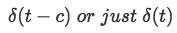
When c=0, the impulse is located at the origin. The impulse is always located at c, so c=0 represents the origin, if this value is different than zero, then the impulse will be located wherever the value of c is at.
Dirac Delta Function properties
Through this section you will find the properties of Dirac Delta function with proofs, or more like, a clarification of each of them. There are three main properties which shed light on how the Dirac Delta function works, and how, correctly speaking, we are talking about a distribution more than a function in the typical sense.
Property 1:
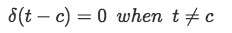
This means that the function had a zero value everywhere except at c. This can also be written as:
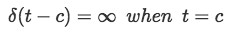
Where you can see that the function has an infinite value only at one point, when t=c, the function is zero throughout the rest of the time (when t ≠ c).
It is important to note that the Dirac Delta function is usually thought as having an impulse value that is infinite. Think on light impulses, just like the beach example, in simple math it would be difficult to quantify how much light you have coming out of the flashlight at an infinitesimally small moment isn't it? And so, we truly do not know this value, thus for practical purposes (and to not just call it "undefined", which could also be done by the way) we say its value is infinite.
Property 2:
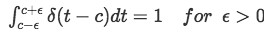
This property represents the incidence of an impulse throughout the graph, in other words, this property means "there is one impulse happening on the range of t that goes from c-ε to c+ε". Therefore, the value of ε must be higher than zero, so you can observe a range of t that is more than just the one moment when the impulse happens (located at c).
Property 2 can also be represented as:
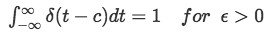
Which basically means that ε has a value of infinity (which would make this integral the same as the one on top). In other words, if we were to integrate the Dirac Delta function through all of the possible values of t (from negative infinity to positive infinity) there would be an impulse at some point in t, which would be in c. This second form is usually used when c=0, since the impulse would be centered at the origin and it would be very easy to see how the range of the integration covers all the negative and positive possible values that t could have with ε=∞.
Property 3:
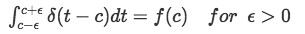
In this case you are multiplying the incidence of an impulse, which is one, to a function and evaluating this function in terms of c.
Paraphrasing the last sentence, this integral means you will have an impulse happening throughout the range of the integration and this impulse is being multiplied to a function (the function can be any function of t), thus you can expect to have a result at the moment of the impulse only. The reason why you will only obtain a value for the function f(t) at c, is that the Dirac Delta function is zero at any other value of t, and therefore at any other value of t, this multiplication yields a zero result too. So, you can only have a result different to zero for f(t) at t=c, which is f(c).
Notice that both property 2 and 3 work for any integration interval containing t=c where ε>0, so the point at which t=c is not one of the edges of the interval. It is also worth noting that just like in property 2, the integral in property 3 can be written having an interval going from negative infinity to positive infinity, since this would mean you are taking into account all of the possible existing values of t, and thus, c must be inside this interval somewhere.
After looking at the properties of the Dirac Delta function we can observe its evident relationship with probability distributions. In simple terms, property two means that the probability of finding an impulse coming from a Dirac Delta function in the range containing c is one, which means 100% probability. In reality, such analysis is much more intricate than this simple explanation but thank to this you can have an idea on how we utilize this particular integral of Dirac Delta in other areas of study. For more information on this topic,visit the next article about using the Delta function in probability and statistics.
For more on the history of the Dirac Delta function and how it came about from studies in Quantum Mechanics, we recommend you to take a look into this paper on the Dirac Delta function identities.
Laplace transform of the Dirac Delta function
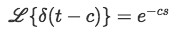
We can compute the Laplace transform of the Dirac Delta function by following the notation from property 3, and so we have:

Observe how this integral is equal to zero at all points of the interval except for t=c.
Therefore, for the simple case in which we have an expression for the Laplace transform of a Dirac Delta function we can solve easily as follows.
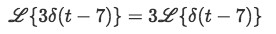
Notice the coefficient can be taken out of the transformation due to linearity.
And so using the general solution we found above:
We solve:
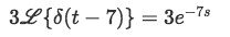
So as you can see, to obtain the Laplace transform of a Dirac Delta function is a straightforward process, and we will use it as a tool to solve more complicated problems.
For that, let us now work through an example problem in which we have initial conditions to solve for a differential equation with a Dirac Delta function included. For this problem we will be using the technique of partial fractions and the table of the inverse Laplace transform results so we recommend you to have these StudyPug sections at hand (maybe in another tab) so you can go and take a look in case you need a quick review.
Example:
-
Solve the differential equation:
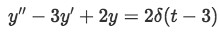
Equation 5: Differential equation containing Dirac Delta function With initial conditions y(0)=1, y'(0)=3
-
First we take the Laplace transform of the whole equation:
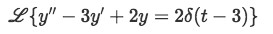
Equation 6: Taking the laplace transform of a differential equation containing Dirac Delta function -

Equation 7: Distributing the laplace transform in the differential equation containing the Dirac Delta function -
To result in:

Equation 8: Simplifying. Taking the laplace transform of a differential equation containing a Dirac Delta function -
Now for the left hand side of the equation we have:
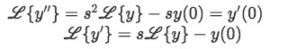
Equations 9 and 10: Laplace transforms of the components of the differential equation containing a Dirac Delta function -
Then plugging these into equation 8:

Equation 11: Substituting equations 9 and 10 into the differential equation containing a Dirac Delta function -
Now plug the initial conditions to simplify:
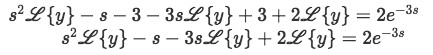
Equation 12: Plugging initial conditions into the differential equation containing a Dirac Delta function -
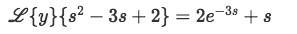
We factorize the Laplace transforms out:
-
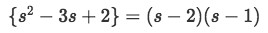
Where we can easily see that:
-
So we have:
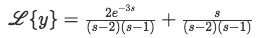
Equation 13: Laplace transform equivalence solved from the differential equation containing a Dirac Delta functio -
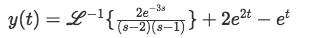
We take the inverse Laplace transform:
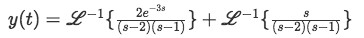
Equation 14: Solution of the differential equation in terms of inverse Laplace transform -
Now let us find the inverse Laplace transform for the two terms in the right hand side of the equation.
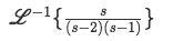
Equation 15: Second right-hand term of the solution of the differential equation in terms of inverse Laplace transform -
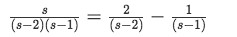
We solve the terms inside the transformation using partial fractions:

Equation 16: Partial fraction expansion -
So:
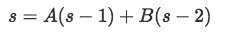
Equation 17: Equation to solve partial fraction coefficients Which is an identity for all values of A and B in this case.
-
In order to solve this last equation we set s equal to a convenient value. Let us set s=1 so:

-
We plug this in the original equation for s and solve for A by setting s=0 now:

-
Therefore equation 16 becomes:
Equation 18: Partial Fraction expansion with coefficients found -
And:

Equation 19: Solution of second right-hand term of the solution for the differential equation (solution for equation 15) Which was solved by checking the table of results for common inverse Laplace transforms.
-
So equation 14 becomes:
Equation 20: Solution of the differential equation in terms of inverse Laplace transform, second right hand term solved -
Now for:
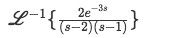
Equation 21: First right-hand term of the solution of the differential equation in terms of inverse Laplace transform -
Solve the terms inside the transformation using partial fractions:

Equation 22: Partial fraction expansion -
So:

Equation 23: Equations to solve partial fraction coefficients -
Set s=1 and this converts into:

-
Knowing that we solve for A by setting s=0

-
So now we know:

Equation 24: First right-hand term of the solution for the differential equation (continuation for equation 21) -
We know from the table of Inverse Laplace transform results that if you get the inverse Laplace of two functions multiplying each other, one in the form of the exponential and one just being a function of s, the result will give a unit step function shifted according the exponent of the original exponential, and the rest will just be transformed properly.
In simple terms, we know that:
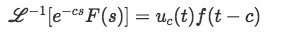
Equation 25: General solution of inverse Laplace transform involving an exponential multiplying a Laplace transform Where uc(t) is the unit step function shifted on c
And f(t) is the inverse Laplace transform of F(s)
In this case: f(t) will be shifted on some constant c, and therefore f(t-c)
-
Therefore, for equation 24:
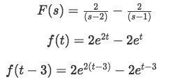
-
So the result for the inverse Laplace transform is:

Equation 26: Solution of first right-hand term of the solution for the differential equation (solution for equation 21) -
And we rewrite equation 20 with this result:

Equation 27: Final solution of the differential equation Which is the final solution for the differential equation.
We suggest to take a look at these Differential Equations notes for more initial value problem Dirac Delta function examples and their properties.
The Dirac Delta function can be thought of as an instantaneous impulse
There are 3 main conditions for the Dirac Delta function:
1.
2.
3.
The Laplace Transform of a Dirac Delta Function is:
We can also relate the Dirac Delta Function to the Heaviside Step Function: