Negative binomial distribution
All in One PlaceEverything you need for better marks in university, secondary, and primary classes. | Learn with EaseWe’ve mastered courses for WA, NSW, QLD, SA, and VIC, so you can study with confidence. | Instant and Unlimited HelpGet the best tips, walkthroughs, and practice questions. |
Make math click 🤔 and get better grades! 💯Join for Free
0/1
Intros
0/3
Examples
Lessons
- Identifying Negative Binomial Distributions
Identify which of the following experiments below are negative binomial distributions?
i. A fair coin is flipped until head comes up 4 times. What is the probability that the coin will be flipped exactly 6 times?
ii. Cards are drawn out of a deck until 2 exactly aces are drawn. What is the probability that a total of 10 cards will be drawn?
iii. An urn contains 3 red balls and 2 black balls. If 2 balls are drawn with replacement what is the probability that 1 of them will be black?
iv. Roll a die until the first six comes up. What is the probability that this will take 3 rolls? - Determining the Negative Binomial Distribution
A fair coin is flipped until head comes up 4 times. What is the probability that the coin will be flipped exactly 6 times? - Determining the Cumulative Negative Binomial Distribution
A sculptor is making 3 exhibits for an art gallery. There is a probability of 0.75 that every piece of wood she carves into will be good enough to be part of the exhibit. What is the probability that she uses 4 pieces of wood or less?


Topic Notes
Negative binomial distribution
When studying the different discrete probability distributions that exist in statistical analysis you will find that some of them share many characteristics and seem to respond to the same problem just with a few shifted things. This is the case for the difference between the binomial and the negative binomial distribution that we will talk about today.
For that, let us go back a little bit and recall what a binomial distribution is, and from that, on the second section of this lesson we will study what the negative version of it is.
What is a binomial distribution?
A binomial probability distribution is a discrete probability distribution which can have two possible outcomes: either a success or a failure; this kind of distribution shows the possible successful results to occur in a series of finite trials and so, the possible outcomes just range between yes and no (did the expected outcome happened? Or did it not?), or true and false, or anything that refers to an event being a success for our result expectation or a failure.
The general probability formula of a binomial distribution (which can be sometimes simply referred as the binomial distribution formula), is defined as follows:
Where:
= number of trials
= number of successes in trials
= probability of success in each trial
= number of success outcomes
= probability of getting successes out of trials
When studying a discrete random variable x and it has a binomial distribution, we are looking for the number of successes in a certain amount of trials. In order to be sure that our statistical experiment is based on such a discrete distribution, there are a few conditions it must meet:
- The experiment has a fixed number of trials. And so, the value of is defined.
- Each trial has only two possible outcomes, the result is either a success or a failure.
- The probability of success for each individual trial is equal.
This last condition is the result of what we call running the trials with replacement, meaning that all of the possible outcomes of the first attempt, are kept for the second, third and nth attempt. No matter how many trials are run, every single one has the same amount and equal possible outcomes, meaning that its probability of success remains the same throughout all of the trials.
Negative binomial distribution
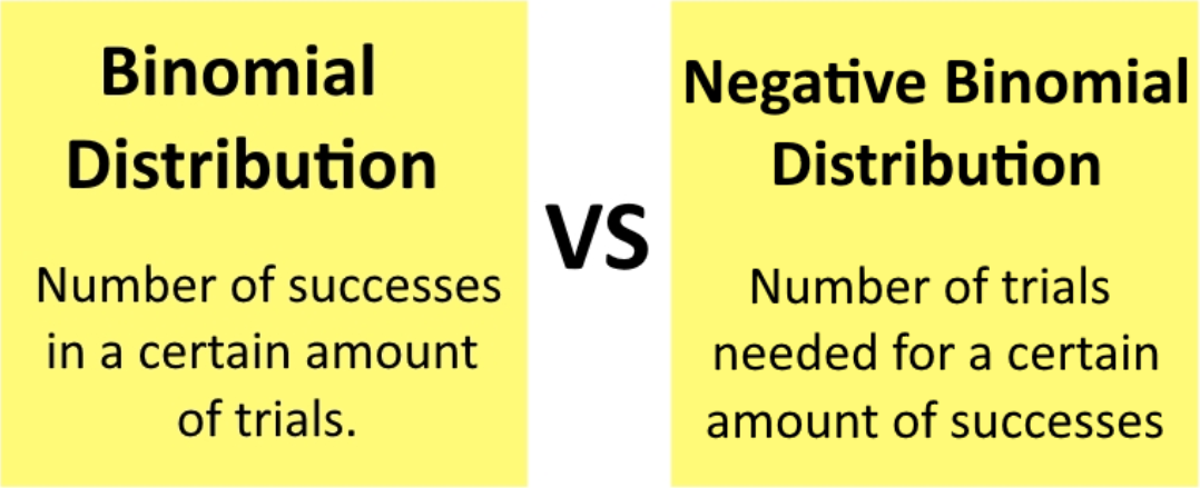
While the binomial distribution is concerned on studying the number of successes in a certain amount of trials, the negative binomial distribution studies the amount of runs in the experiments that have to pass so a certain number of successes occur. Just as in the binomial distribution, the negative binomial distribution has only two possible outcomes in each trial: either a success or a failure.
Just as the binomial distribution, the negative binomial distribution has certain conditions:
- There are only two possible outcomes for each trial in the experiment.
- The probability of success in each trial is constant, in other words, it doesnt matter how many trials are run in the experiment, the value of the probability of success in each is the same.
- There is a set number of trials to run in the experiment, and each of these trials is independent from the others.
With that in mind, the negative binomial distribution equation for probability is defined as
Where:
= number of trials
= number of successes in n trials
= probability of success in each trial
= probability combinations for successes
= probability of getting successes out of trials
Do not confuse the probability of the negative binomial distribution thinking this means the probabilities calculated are negative! There is no such thing as a negative probability! This distribution has the word negative on its name given the nature of the perspective by which the problem is looked at, kind of a backwards perspective when comparing it to the binomial distribution, and thus the name.
Negative binomial distribution examples
Using the negative binomial definition as presented above, let us work through a few examples to gain practice:
Example 1
We start with an example focused on knowing when you have negative binomial distributions presented to you. And so, identify which of the following experiments below are negative binomial distributions, we recommend you to use the three conditions mentioned on our last section, plus figure 1, so you do not confuse them with simple binomial distributions. A fair coin is flipped until head comes up 4 times. What is the probability that the coin will be flipped exactly 6 times?
This is a typical example of a negative binomial distribution since the problems asks about the number of trials needed in order to obtain a certain amount of successes.
Cards are drawn out of a deck until 2 exactly aces are drawn. What is the probability that a total of 10 cards will be drawn?
Although this problem asks for the chances of a certain number of trials to be done in order to reach the successes desired, this is not a negative binomial distribution because every time a card is drawn, the probability of success of each trial changes. So if the probability of success in each trial is not constant, this cannot be a negative binomial distribution.
An urn contains 3 red balls and 2 black balls. If 2 balls are drawn with replacement what is the probability that 1 of them will be black?
This is not a negative binomial distribution example, since the problem asks about the probability of a certain amount of successes per two trials: therefore this is a binomial distribution.
Roll a die until the first six comes up. What is the probability that this will take 3 rolls?
This is not a negative binomial distribution because the problem focuses in an experiment that will go on until the first success occurs; as we learnt in our past lesson, this is a geometric distribution.
Example 2
On this negative binomial example we focus on calculating the distribution using the equation for the probability defined in equation 2.A fair coin is flipped until head comes up 4 times. What is the probability that the coin will be flipped exactly 6 times?
For this case we have that:
number of times the coin will be flipped.
number of successes we want.
the probability of success in each trial must be one half since there are 50% chances a particular face comes up when flipping a coin.
which makes sense, since there are 50% chances of success in each flip, there are 50% chances of a failure in each flip.
And so, we calculate the probability that the coin will be flipped 6 times and we will obtain 4 successes:
Therefore, there are 15.625% chances of flipping a coin six times and obtaining four successes on that run.
Example 3
Determining the Cumulative Negative Binomial DistributionA sculptor is making 3 pieces to exhibit at an art gallery. There is a probability of 0.75 that every piece of wood she carves into will be good enough to be part of the exhibit. What is the probability that she uses 4 pieces of wood or less in order to produce the 3 final to exhibit at the gallery?
For this case we have that:
number of pieces of wood she will use to obtain the final carved pieces to exhibit..
number of successes we want.
the probability of each carved piece to be part of the sculptors exhibit.
is the probability of a piece not to be used in an exhibit.
In this case it is important to note that n cannot have a value of zero, actually, it cannot have a value smaller than three since the sculptor MUST use at least one piece of wood to produce one piece of art. Therefore n is less or equal to 4, but is higher than 3 for this case.
And so, we calculate the cumulative probability, for using four pieces of wood or less, which means that we have to add the probabilities of the sculptor using three and four pieces of wood:
Therefore, we calculate the probability for the different values of separately:
Therefore the final result for the probability is:
So now that you have learned the negative binomial distribution definition and worked through a few problems, you are ready for the last discrete probability distribution we will see in this course: the hypergeometric distribution.
But before that, let us recommend you some other study materials: on this negative binomial distribution lecture you can find an example for negative binomial variance and mean. On this lesson on the hypergeometric and negative binomial distributions you can see the relationship between these two and the simple binomial distribution, and their differences, such lesson can serve as an introduction to our next one.
And so, this is it for today, we hope you enjoyed this lesson, and see you in the next one!.
• Negative Binomial Distribution:
: number of trials
: number of success in n trials
: probability of success in each trial
: probability of getting the success on the trial
: number of trials
: number of success in n trials
: probability of success in each trial
: probability of getting the success on the trial