Hypergeometric distribution
All in One PlaceEverything you need for better marks in university, secondary, and primary classes. | Learn with EaseWe’ve mastered courses for WA, NSW, QLD, SA, and VIC, so you can study with confidence. | Instant and Unlimited HelpGet the best tips, walkthroughs, and practice questions. |
Make math click 🤔 and get better grades! 💯Join for Free
Intros
Examples
Lessons
- Identifying Hypergeometric Distributions
Identify which of the following experiments below are Hypergeometric distributions?
i. Negative Binomial – A 12 sided die (dodecahedra) is rolled until a 10 comes up two times. What is the probability that this will take 6 rolls?
ii. Binomial – An urn contains 5 white balls and 10 black balls. If 2 balls are drawn with replacement what is the probability that one of them will be white?
iii. Hypergeometric - A bag contains 8 coins, 6 of which are gold galleons and the other 2 are silver sickles. If 3 coins are drawn without replacement what is the probability that 2 of them will be gold galleons?
- Determining the Hypergeometric Distribution
A bag contains 8 coins, 6 of which are gold galleons and the other 2 are silver sickles. If 3 coins are drawn without replacement what is the probability that 2 of them will be gold galleons? - Determining the Cumulative Hypergeometric Distribution
Ben is a sommelier who purchases wine for a restaurant. He purchases fine wines in batches of 15 bottles. Ben has devised a method of testing the bottles to see whether they are bad or not, but this method takes some time, so he will only test 5 bottles of wine. If Ben receives a specific batch that contains 2 bad bottles of wine, what is the probability that Ben will find at least one of them?


Topic Notes
Hypergeometric distribution
Hypergeometric distribution definition
The hypergeometric distribution is a discrete probability distribution that looks to study the probability of finding a particular number of successes for a certain amount of trials done during a statistical experiment. While the rest of the discrete probability distributions we have seen so far operate on probability with replacement, the hypergeometric distribution does not follow that same behavior.
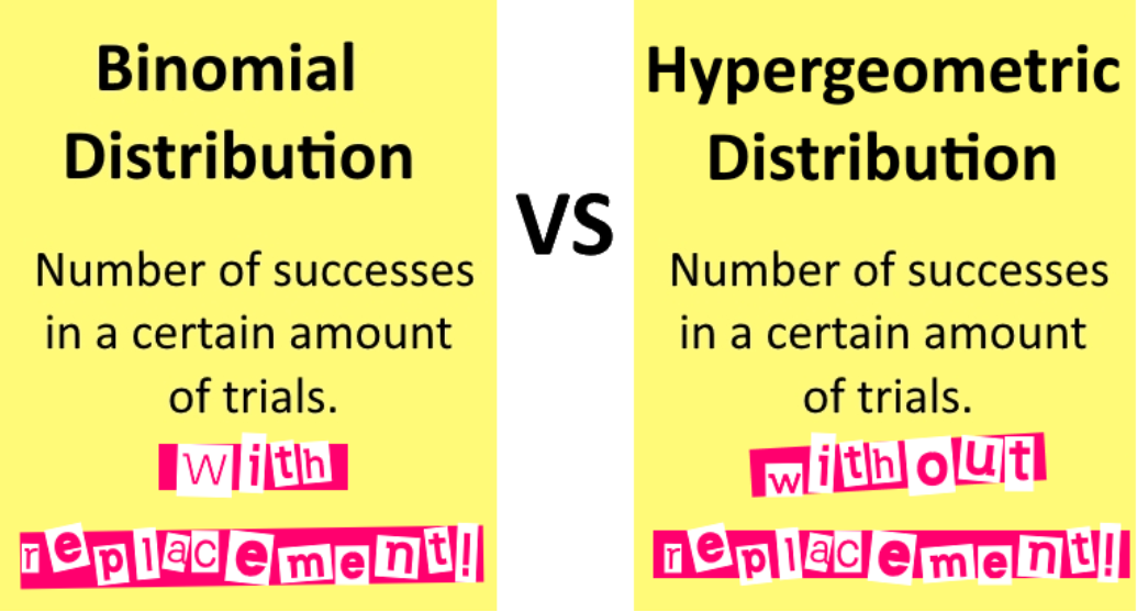
Due its name, you may think the hypergeometric distribution is easily comparable with the geometric distribution; funny enough, it is actually much more easy to compare it with the binomial distribution!
At this point you may have already noticed the similarities between the binomial and the hypergeometric distribution definition, they are ALMOST the same, there is just one bit part that differs from one to the other: one uses sampling with replacement and the other one without replacement, which changes the probability of success in each attempt from constant (when replacement is used) to a changing value (without replacement).
Given that there will be no replacement on the hypergeometric distribution, in order for a statistical experiment data to be following such kind of distribution it must meet the next requirements:
- Having a total population, a sample of fixed size is picked from it at random without replacement.
- In both the population and the sample, there are just two different kinds of outcomes: successes and/or failures. A success is the outcome you want to obtain, or are specifically studying.
- The probability of a success in each trial is not constant. Since items in the sample are randomly selected without replacement, the amount of successes left in the sample changes from one trial to the next and so the probability changes.
And so, the hypergeometric distribution formula for the probability is defined as:
Where:
= population size
= number of successes in the population
= sample size
= number of successes in the sample
= probability of getting x successes out of a sample of trials
Notice that for this particular distribution, you should completely understand how to work with the binomial coefficient formula, or also called the combinations formula. In later lessons we will take a look into the details of combination examples, for now, we have been providing you with the already defined formulas throughout all of the definitions of the different discrete probability distributions.
How to calculate hypergeometric distribution
When calculating the probability without replacement as the hypergeometric distribution requires, we need to take into account the difference between the total population and the sample items.
Example 1
For our first hypergeometric distribution example, we will be determining the probability in the next case:A bag contains 8 coins, 6 of which are gold galleons and the other 2 are silver sickles. If 3 coins are drawn without replacement what is the probability that 2 of them will be gold galleons?
For this case we have:
. Therefore, we calculate the binomial coefficients for each of the combinations needed in the probability formula as shown in equation 1:
And using these results, we work through the probability for the hypergeometric distribution calculation:
Example 2
On this example, we are to determine the cumulative hypergeometric probability of the next experiment:Ben is a sommelier who purchases wine for a restaurant. He purchases fine wines in batches of 15 bottles. Ben has devised a method of testing the bottles to see whether they are bad or not, but this method takes some time, so he will only test 5 bottles of wine. If Ben receives a specific batch that contains 2 bad bottles of wine, what is the probability that Ben will find at least one of them?
Therefore, the probability that Ben finds at least one bad bottle of wine must be the addition of the probability of Ben finding one bad, plus the probability of Ben finding two bad bottles:
On this case, we have that the population size, the number of successes in the population and the sample size are constants, which have the following values: and .
We start by calculating the probability of finding one bad bottle, which means that the number of successes in the sample is equal to 1 or just .
Now calculating the probability of finding 2 bad bottles of wine, therefore :
Therefore, the probability that Ben finds at least one bad bottle of wine is:
Hypergeometric test
The hypergeometric test is the usage of the calculation of cumulative hypergeometric probabilities in order to see if a statistical process result is realistic or contains a certain kind of bias. In other words, when drawing a sample from a population, depending on the original conformation of the population (how many possible successes and failures it contains), we should have an idea of the quantities of successes we may draw within our sample because of the proportions in the population. But sometimes, the sample may not truthfully represent the original population and that is usually the sign of some kind of bias.
Remember, bias means, the experiment is not done randomly, there is either a systematic error or a particular characteristic in the way how the sample was drawn that provides a sample uncharacteristic of the population we are using.
Therefore, the hypergeometric test is a tool to decide if the sample we drew from a population is good or not. When the sample contains many more successes in proportion to the ones found in the original population, this is called over-representation, and we can obtain the probability of this happening by calculating the cumulative hypergeometric probability of us drawing the particular amount of successes drawn and more. If the sample contains much less successes in proportion to the ones found in the original population, then this is under-representation, and we obtain the probability of this happening by calculating the cumulative hypergeometric probability of us drawing the particular amount of successes drawn or less. If such probabilities are way too low, we can decide the sample we drew is biased and therefore, not representative of the population (if working on something like demographics) or just finding that our experiment is not random and has something going on that messes up with the probabilities.
To finalize the lesson for today, let us provide you with some recommendations:
This handout on the hypergeometric and negative binomial distributions provides a wide variety of examples for both types of distributions and well explained summarized introductions for each. Then, this other document presents a clear comparison between the binomial and the hypergeometric distribution on the first page, and the continues onto examples. Both of these links are great materials that can be helpful to continue your studies on this topic.
This is it on all of the discrete probability distributions we will present on our statistics course, to finish, let us present you with a table where you can see all of them summarized:
Table of Discrete Probability Distributions
|
Distribution definition: |
Characteristics: |
Probability formula: |
|
Binomial distribution: Number of successes in a certain amount of trials (with replacement) |
Fixed number of trials. Each trial has only two possible outcomes: a success or a failure. The probability of success in each trial is constant. |
Where: = number of trials = number of successes in n trials = probability of success in each trial = number of success outcomes = probability of getting x successes out of n trials |
|
Poisson distribution: Used as an approx. to the binomial distribution when the amount of trials in the experiment is very high in comparison with the amount of successes. |
Fixed number of trials. Each trial has only two possible outcomes: a success or a failure. The probability of success in each trial is constant. |
→ Where: = number of trials = number of successes in n trials = probability of success in each trial = probability of getting x successes out of trials average number of events per time interval |
|
Geometric distribution: Number of trials until the first success. |
Fixed number of trials. Each trial has only two possible outcomes: a success or a failure. The probability of success in each trial is constant. |
Where:
= number of trials until the first success
= probability of getting your 1st success at trial |
|
Negative binomial distribution: Number of trials needed for a certain amount of successes. |
Fixed number of trials. Each trial has only two possible outcomes: a success or a failure. The probability of success in each trial is constant. |
Where: = number of trials = number of successes in n trials = probability of success in each trial = number of success outcomes = probability of getting successes out of trials |
|
Hypergeometric distribution: Number of successes in a certain amount of trials (without replacement) |
A randomly selected sample of fixed size is selected without replacement from a population. The population and the sample have only two possible outcomes: a success or a failure. The probability of success in each trial is not constant. |
Where: = population size = number of successes in the population = sample size = number of successes in the sample
|
m: number of successes in the population
n: sample size
x: number of successes in the sample
P(x): probability of getting x successes (out of a sample of n)